
To Add Calculated Fields in Google Sheets
- Click on a value cell.
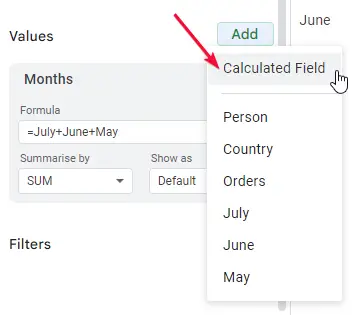
- In the editor, under “Values,” click “Add” > “Calculated Field“.
- Define a formula for the calculation (e.g., to calculate the sum of three months, use “=July+June+May“).
- Choose between “Sum” (for all rows) or “Custom” (for specific rows).
- Rename the calculated field for clarity.
Hi guys, in this article we will learn about how to add calculated fields in Google Sheets.
Calculated fields are a part of pivot tables, and they are very important when working with pivot tables. When using pivot tables, we use a different kind of its feature to summarize our data in many different ways, we can sort the tables, can display the sum of the column, can use many available functions for the selected columns, and many other things. But when we need to use a custom range of columns, we don’t have a direct method but a calculated field that helps us to add a column and perform a custom calculation in it to get useful insights about the data.
We need to have a pivot table to use the calculated field feature and to have a pivot table we should have some data. So, in this article, we will see the entire process from start to end to learn how to add calculated fields in google sheets.
Use of Calculated Fields in Google Sheets
We use pivot tables to draw handy and quick useful insights into the data. We may have a large dataset that has various rows and columns, we have the power to use specific columns and find the average, sum, count, and many of these functions. But we cannot find out the values of more than one column directly, in the values section of the pivot tables we have a “add” button that can add only the columns that exist in our data, to add a column with a function that performs some calculation on various columns, we need calculated field, now you got it.
We need the calculated field as a new column in our pivot table to make it more useful and get any possible calculator to get useful and helpful insights to analyze the data. We can use many of the given functions, aggregate functions, and also a custom formula to perform the calculation on a calculated field. This is why we need to learn how to add calculated fields in google sheets. In this article, we will add multiple calculated fields in the pivot table to see how it works and how it behaves in different conditions.
How to Add Calculated Fields in Google Sheets
Here we will learn the step-by-step procedures to add calculated fields in google sheets. We will first create some sample data, then we will generate a pivot table using that data, and then finally we will add some calculated fields to our pivot table, in this way you will completely understand how it works.
So, let’s get started.
How to Add Calculated Fields in Google Sheets – The Sample Dataset
First, we need some sample dataset to generate a pivot table, for data, there are no specific rows and columns required, you can have any number of rows and columns that are generally meant to be added to generate a pivot table.
Step 1
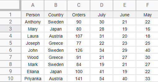
Make some sample data (make similar data so you can follow and practice the example)
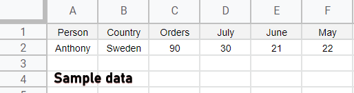
Step 2
Add person name, country, orders, and last three months’ order (this will make it easy to add maximum calculated fields for your practice)
Now we need to make a pivot table using this table, let’s see that in the next section.
How to Add Calculated Fields in Google Sheets – Making a Pivot Table
In this section, we will see how to add calculated fields in google sheets and making of a pivot table. Making it very simple.
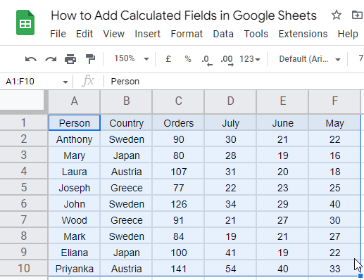
Step 1
Select all the data including headers
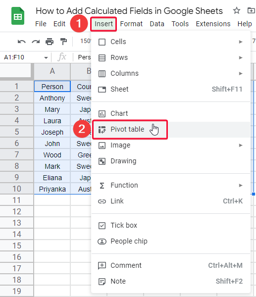
Step 2
Go to Insert > Pivot Table
Step 3
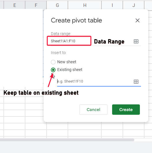
A dialog box will appear, select one radio button option from “New sheet”, or “Existing sheet”, and it will add the table on the new sheets or existing sheet respectively.
Step 4
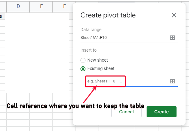
Now it will ask for a cell address in the below input field, pass a cell reference where you want to locate your pivot table. Let’s say “Sheet1!G1”, simply click on the cell and it will be selected.
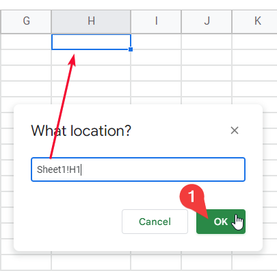
Step 5
Now, it will further confirm the given cell address, verify and Click on Ok to add the pivot table.
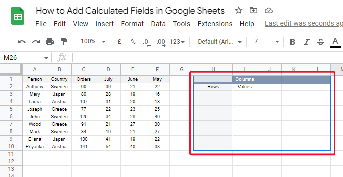
Step 6
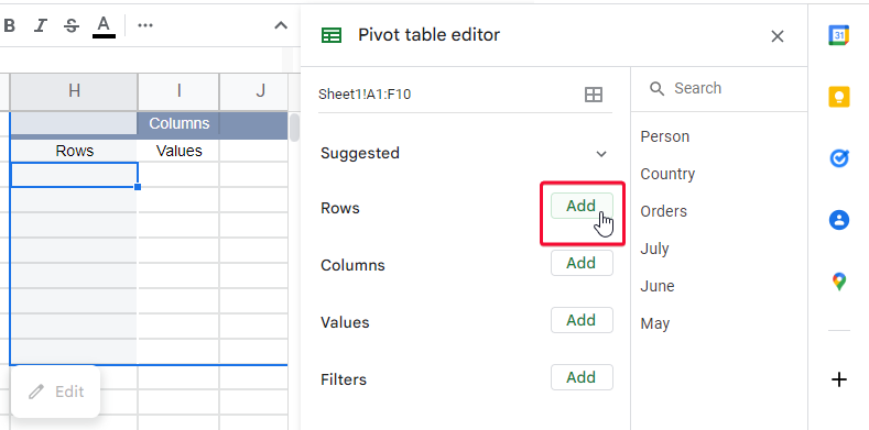
A basic template will be added, now you have an editor box on the right-hand side, you can play with it to perform certain actions.
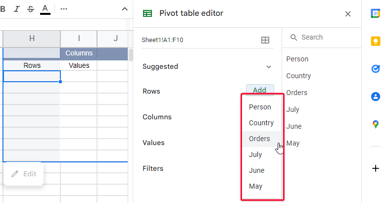
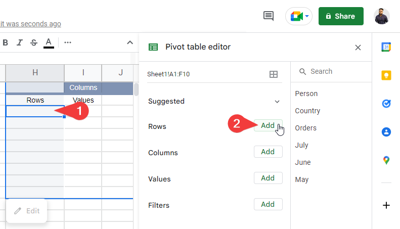
Step 7
Adding a row into a pivot table
Step 8
Calculating the sum of values for each row
Step 9
Calculating the single values for each row
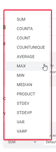
Step 10
Using various functions
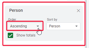
Step 11
The sort features.

These were some basic features you can use in a pivot table or editor. I hope you have got a basic idea of how the pivot table works.
Now let’s move and see what’s the rule of calculated fields here in the pivot table.
Why do we need Calculated Fields inside Pivot Table in Google Sheets?
We have seen various methods in the pivot table in previous sections, we have seen how to sort, sum, count, and use other functions within the pivot table, but there is a term called “calculated field” for the sum or more than one column that does not have an original column in the source data, we will make a newly generated table (inside the pivot table) named as calculated field and we can perform any kind of calculation in it. We can also rename this column later. So, let’s consider a scenario, in our data, we have a total number of orders and the orders of the last three months in different columns. what if we need to see the difference between the last three months’ order and the total order, we don’t have any direct method to do this. Similarly, there are many use cases, let’s see them practically
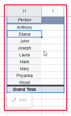
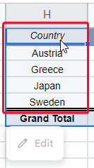
Step 1
Click in a row-column, and add some rows (from your existing data)
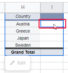
Step 2
Select a value column cell
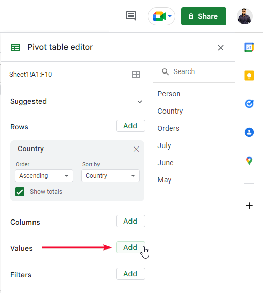
Step 3
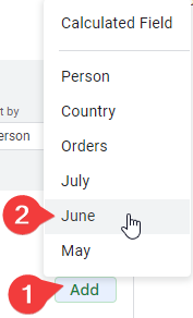
In the Table editor, go to values, and click on the “add” button next to values.
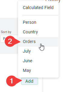
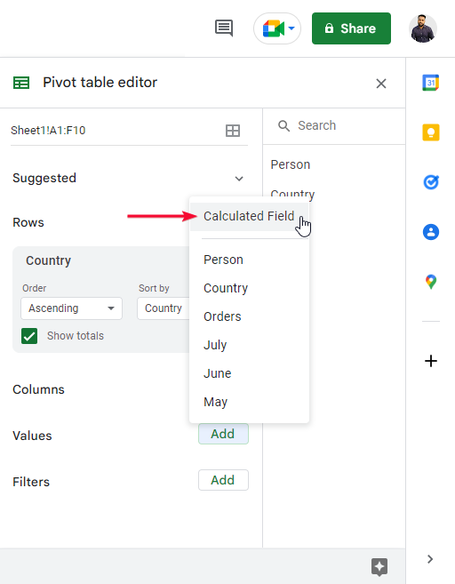
Step 4
Click the calculated field from the given options
Step 5
Now, you will need to provide the formula based on which the calculation will take place.
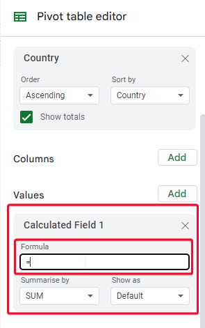
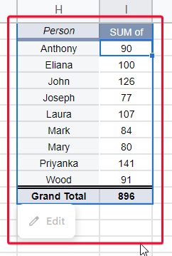
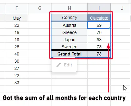
Here, let’s assume we want to calculate the sum of all three months.
Step 6
We will add a custom formula for it
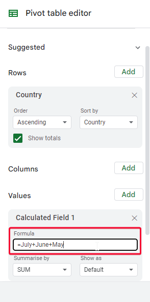
=July+June+May
Note that, there should not a spelling mistake, the column header’s name should be the same.
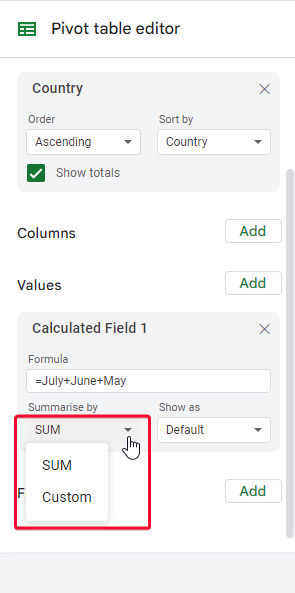
Step 7
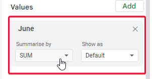
Choose “sum”, or “custom” from the below dropdown
Sum: to sum all the rows
Custom: to sum only the tied rows
Step 8
Rename the column with a meaningful name, and you’re done.
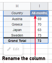
This is how to add calculated fields in google sheets.
Let’s see another quick example.
Another Example:
In this example, we will find out another calculated field.
See the below screenshots.
Step 1
Click on value > Add > calculated field
Step 2
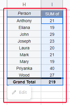
Define the formula, here I am going to use
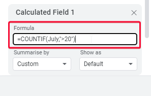
=COUNTIF(July,”>20″)
Here July is the column header in my original data.
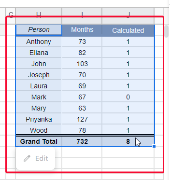
Step 3
The result
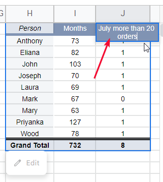
Step 4
Give this calculated field a meaningful name too.
This is how you do this, you can calculate as many calculated fields as you want, note that you need to use the formula having the original column reference and not a reference of a calculated field column.
Download/Copy Google Sheets Workbook
Notes
- We need to write accurate column names (spellings, caps, and spacing)
- If your column header name has more than one word then you can use it inside single quotes.
- You cannot use a column that is generated inside the scope of the pivot table to add more calculated fields, in simple words, you cannot find a calculated field using a calculated field.
FAQs
How to add calculated fields in google sheets?
Calculated fields are the part of pivot tables in google sheets, we can calculate many things using several functions within the pivot table but when it comes to performing some calculations on various columns than we need to use calculated fields, as I have shown in the above methods and examples, we can add calculated fields in google sheets by clicking on the add button placed after the values section. Note that, we cannot find out more calculated fields using previously calculated fields, but we can rename these fields.
Can I use calculated fields other than pivot tables?
No, calculated fields are part of pivot tables in the context of google sheets, we have a pivot table first then inside pivot tables we can use the features of calculated fields. No outside the pivot table in google sheets.
Conclusion
Wrapping up how to add calculated fields in google sheets, we have learned what are calculated fields, what are pivot tables, where we can find the feature of calculated fields, and how it helps us perform the calculations. We have first seen the data that is used to generate a pivot table, then we moved ahead and learned how to generate a pivot table using that data set, then we did some basic functions to teach you how to pivot table works and how useful they are, then we saw two scenarios in which first we perform a calculation to add a calculated field, then we rename the column and we added another calculated field in which we used some other column and condition, so this is how we can add calculated fields in google sheets. I tried to cover everything in the context of this article.
That’s all from how to add calculated fields in google sheets. I will see you soon with another great tutorial, till then take care. Don’t forget to share, like, and subscribe to the Office Demy blog. Keep learning with Office Demy. Thank you.
