How to Apply Conditional Formatting Lowest and Highest Value in Google Sheets

In this article, we will discuss how to apply Conditional Formatting Lowest and Highest Value in row Google Sheets.

What is Conditional Formatting Lowest and Highest Value in row Google Sheets

Conditional Formatting allows us to automatically apply certain formatting styles based upon certain conditions and formulae. So that we do not have to look at all the values in sheet to find certain values rather as long as they get highlighted due to conditional formatting, they will appear more visible to the eye and are quite easy to find. Google Sheets also provide us formulae to find Minimum and Maximum of a set of values so we can apply Conditional Formatting Lowest and Highest Value in row Google Sheets to find MIN and MAX of a row in Google Sheets.

Why we use Conditional Formatting Lowest and Highest Value in row Google Sheets

We deal with large amounts of data in Google Sheets. The values may exceed hundreds or thousands number of cells. In such cases, to find the minimum and maximum value is a very troublesome task. Doing it by hand can take hours and still if the values of the cells change. The user has to check all the cells again. So for this purpose, we use Conditional Formatting Lowest and Highest Value in row Google Sheets. The method for applying Conditional Formatting Lowest and Highest Value in row Google Sheets is explained in a very easy and understandable manner below.

Download/Copy Practice Workbook

How to use Conditional Formatting Lowest and Highest Value in row Google Sheets

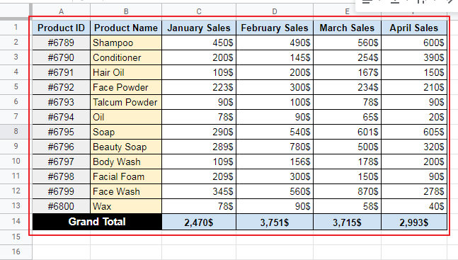
Let us consider the scenario where we have the products information of sales for various months of sales in dollars. Now we need to find out the maximum and minimum month of sales for better evaluation of products sales per time. We can achieve this using method of Conditional Formatting Lowest and Highest Value in row Google Sheets.

We will highlight the lowest sales value in Red Bold Text and maximum sales value in Green Bold Text for better visual.

Suppose we have the following Google Sheet:

Step 1:

Select the cells for applying Conditional Formatting.

Here, Select the row of “Grand Total” of sales cells where we have to find the minimum and maximum formatting as:

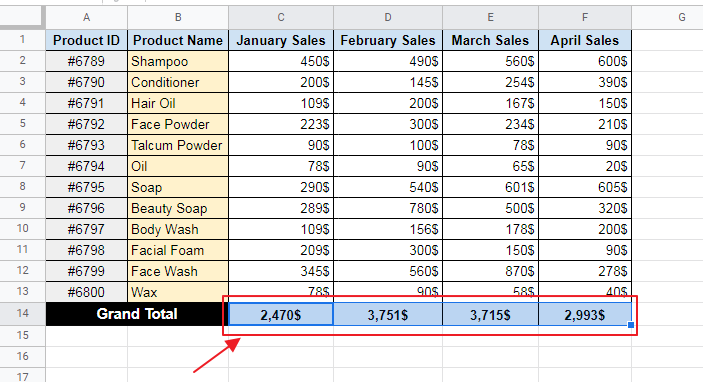
You will see as you select the row, it starts to appear as blue implying these are selected cells.

Step 2:

Apply Conditional Formatting using one the methods below:

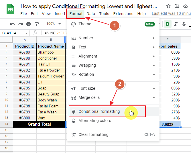
• Method 1:
  • You can click on Format Toolbar and then select Conditional Formatting using steps below:
  • Format Toolbar -> Conditional Formatting

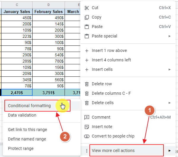
• Method 2:
  • Right Click on the selected cells, a sub-menu will appear. Choose “View more cell actions” and then finally Conditional Formatting using method below:
  • Right Click -> View more cell actions -> Conditional Formatting

Conditional Formatting Rules Box will appear as:

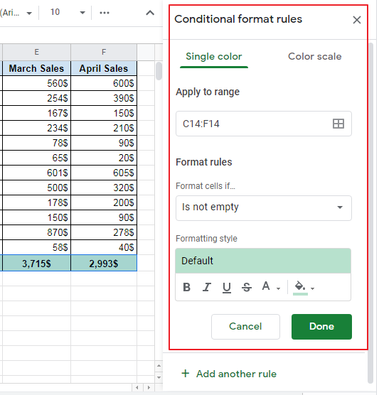
Step 3:

Now, write down the condition(s) that is required to be satisfied in order to perform conditional formatting.

In this case, there are two rules; minimum value in row and maximum value in row. We will highlight maximum value of sales in Grand Total row using Green Bold Text and minimum value of sales in given months as Red Bold Text for better visual.

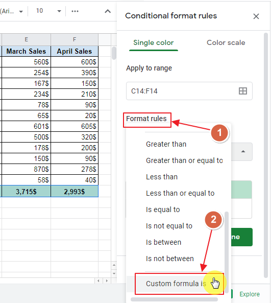
We need to specify condition to get the maximum value out of the row. Condition can be written in the Conditional Formatting Rules Box using the method:

Format Rules -> Format Cells If -> Custom Formula Is

Steps are as:

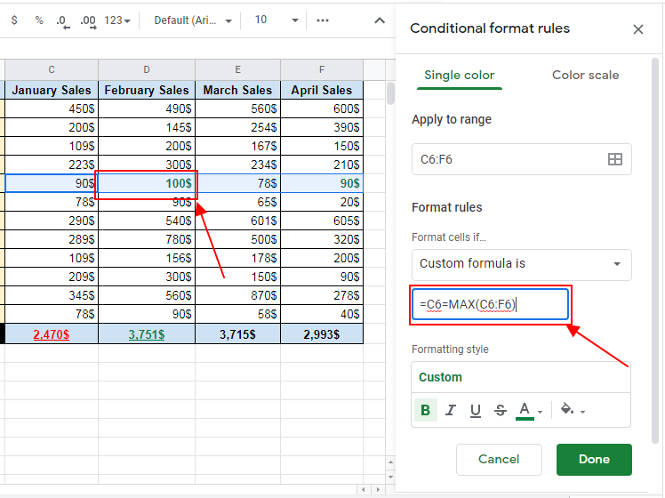
Now, write down the formula for finding the maximum sales value of row as=C14=MAX($C$14:$F$14)” in Format Rule ; Value or Formula Box as:

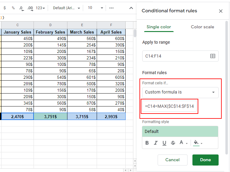
As you finish writing the formula. You can see that out of the selected cells, the cell having the highest value for is following the default Conditional Formatting Format.

Step 4:

As the condition has been set, now is the time to set the format we require for conditional formatting.

Here, we want the highest value to have Green Bold Text. We set it under the Formatting Style section as:

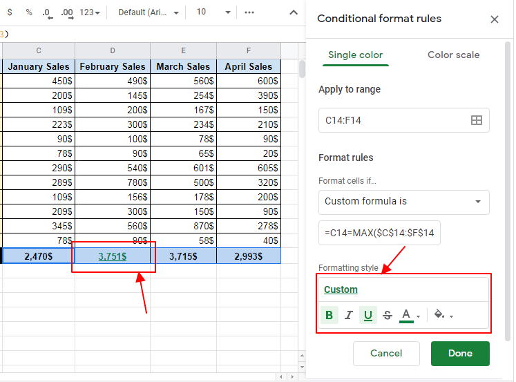
We see on left side that highest value is turning to our desired format which confirm even more that our formula is correct.

Step 5:

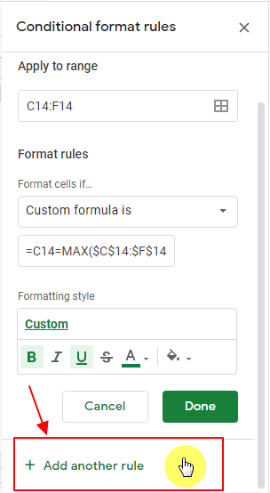
Now click “Add another Rule” under the Conditional Formatting Rules Box to set the next rule for minimum value of sales in the row as:

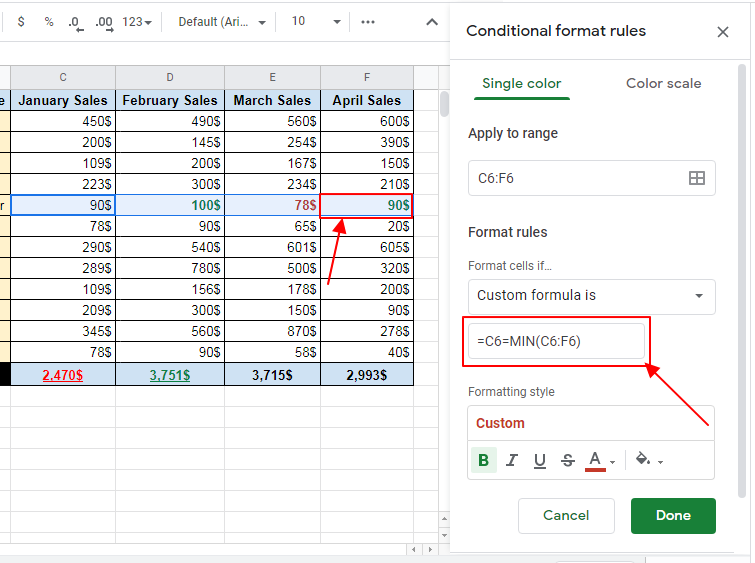
Now, as the rule for finding the maximum sales value in row is set, the next rule for highlighting the minimum value of sales in row is set using the formula “=C14=MIN($C$14:$F$14)” as:

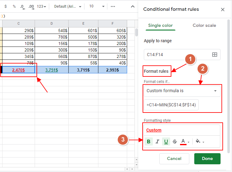
You can see that the changings are applying as we type the formula and set the formatting style.

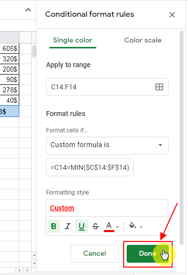
Step 6:

Now, click “Done” to submit the conditional formatting or “Cancel” to cancel it if it is not required Conditional Formatting.

You can see that we get the output as:

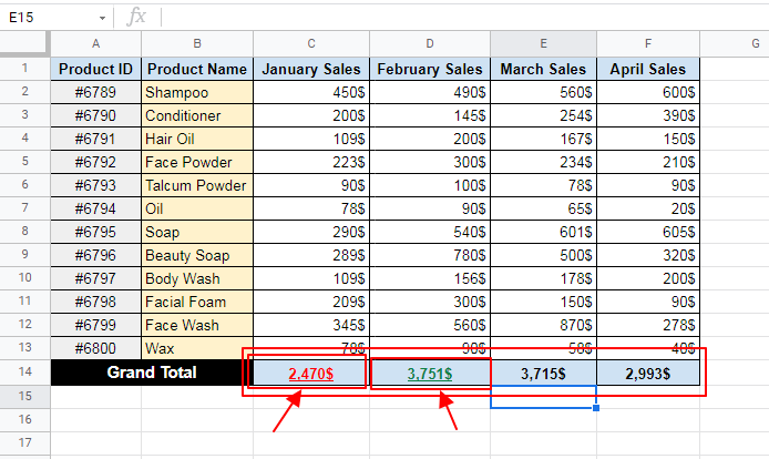
Which is the required result.

Notes

The formula used “=C14=MAX($C$14:$F$14)” has a shortcoming that it uses the absolute values of cells (showing in $ sign) and hence cannot be copied for other rows rather the cells numbers have to be manually changed which defeats the purpose of using Google Sheets for automation.

We used the formulae as “=C14=MAX($C$14:$F$14)”, while another alternative could have been =C14=MAX(C14:F14). But there is an issue with this alternative. Although it looks easy and formula does seem correct. In actual, using such formula can lead to false results.

Let us see what happens when you apply this seemingly correct formula to above rows:

We put the first part of conditional formatting to get the highest value. Now let us apply for lowest value in row as:

We can see that more than one cells are being highlighted for highest value although this is not the case here. So we better use the formula with absolute values as described above. Or another alternative is to use “Color Scale” in Conditional Formatting.

Conclusion

Conditional Formatting Lowest and Highest Value in row Google Sheets allows us to find minimum and maximum value’s cells in large sheets which enables us to find more about our own business (or data) automatically rather than going through thousands of cells and save up a lot of time of user. In this article, method for finding minimum and maximum value in row is described. Any queries are most welcomed. Feel free to comment below for any questions.

Thanks for Reading!