FIX Formula Parse Error in Google Sheets [Guide 2023]

In this article, we will learn about the common Formula Perse Error in Google sheets. We will also provide the solution on how to fix Formula Parse Error in Google Sheets with real-life examples.

What is Formula Parse Error in Google Sheets?

Google Sheets allow us to use formulae in order to save up precious time of user. Rather than spending time on doing the mathematical and logical calculations manually, users can just use automated formulae and functions in their worksheets to get desired results. While using formulae and functions, users may get errors instead of required results. There are different types of errors while parsing formulae in Google Sheets, collectively called Formula Parse Errors of Google Sheets.

As there are multiple types of formula parse error in Google Sheets, there are also various different reasons for existence of each one. It gets more and more complicated to figure out the reason for error with the expansion of the formula. In this article, we will discuss various types of formula parse errors in Google Sheets, along with their reasons and correction methods.

Types of Formula Parse Errors in Google Sheets

Although Google Sheets also display a short error message when error occurs which may help in finding out the reason for error. Let us discuss a few formula parse errors briefly before going onto reasons of their occurrences and correction procedures.

There are multiple formula parse errors in Google Sheets. Some of them are as:

#ERROR! Error

#ERROR! Error may occur when you are following the correct syntax of Google Sheets but your formula does not amount to anything.

An example of such type of error is giving empty parenthesis inside formula. Although you are allowed to use nested parenthesis in Google Sheets, those parenthesis being empty does not mean anything in Google Sheets. Say you used a formula =SUM(B1:B3,()); although the formula is with correct syntax still empty parenthesis confuse Google Sheets on what you want to achieve so you will get a #ERROR error.

#DIV/0! Error

This error means exactly what it says, i.e. DIV/0 means dividing a number by 0.

An example of such type of error is when you are dividing numbers and denominator turn out to be zero. For example, =9/(-2+2) will result in a DIV/0! Error.

#VALUE! Error

VALUE! Error occurs when formula contains an invalid value or the value which is not in the specified format required by the formula.

An example of such type of error is when you try to add up two cells say =C5+D5 while C5 is an integer value while D5 is a text or string value. Then, #VALUE! Error will show up.

#N/A Error

N/A is one of the most occurring error in Google Sheets.

We know that N/A stands for “Not Applicable”. This is the same definition for N/A in Google Sheets as well. When Google Sheets cannot find what it is looking for, it will give this NOT APPLICABLE (N/A) Error.

An example of such type of error is when you are using a VLOOKUP function to find a value which does not exist in the range at all.

#REF! Error

REF stands for “reference” here. Getting REF! Error means that you have referenced a cell or range in formula that does not exist at all.

An example of such type of error is that you specified the range R3:R9 but one or more cells of this range has been deleted. As long as Google Sheets find the referenced cells, it would not give this error rather display the results.

#NAME? Error

NAME? Error occurs when formula contains an invalid name that Google Sheets cannot find and hence the formula results in an error.

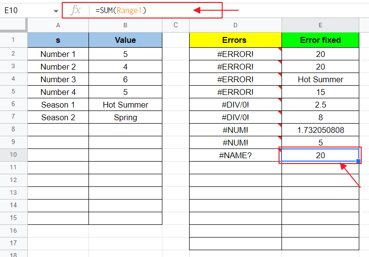
An example of such type of error is when you have a named range called “range01” but you mistakenly write a formula =SUM(range1) in your formula box. As Google Sheets cannot find the named range range1, then it will give a #NAME? Error.

#NUM! Error

NUM! Error occurs when you are trying to display a number which is either too big to calculate and display. For example, =8767263978626783687*39273847293098982903; but this reason for the occurrence of NUM! Error is fixed by Google Sheets. Now, the Google Sheets would display too big results in the form of 3.44324E+38 rather than giving #NUM! Error.

But there is a possibility that #NUM! Error may still occur. If your formula contains a numeric value which is invalid, #NUM! may still occur.

An example of such type of error is when you are trying to find square root of a negative number; it results in an invalid number. Although you can still find the square root of negative numbers by the use of complex calculations using imaginary numbers.

Another example is when you are trying the find the 6^th smallest member of the range while there are only 5 elements in the range.

How to fix Formula Parse Error in Google Sheets

If you deal with Google Sheets on a regular basis, you must have encountered lots of formula parse errors. As some common examples of the formula parse errors are given above; let us discuss these errors and a few more errors in details.

Why we get #ERROR! Error in Google Sheets

We may get #ERROR! Error in Google Sheets when we are trying to achieve something useful with the correct syntax but the formula itself does not amount to anything. For example, you may write a SUM function with a nested parenthesis as =SUM(()); although it has the correct syntax as SUM contains a parameter () but it is empty and so Google Sheets cannot fetch any value from it.

Common causes of #ERROR! are:

• Empty brackets inside formula
• Number of closing brackets is not equal to number of opening brackets in formula.
• Missing “,” comma or “:” colon

When we write the formula as:

Submitting this formula would result as:

Another example may be when you give SUM two parameters; one parameter that is a valid range while the other one is an empty parenthesis which has no actual value but is still working as a parameter which returns no value as:

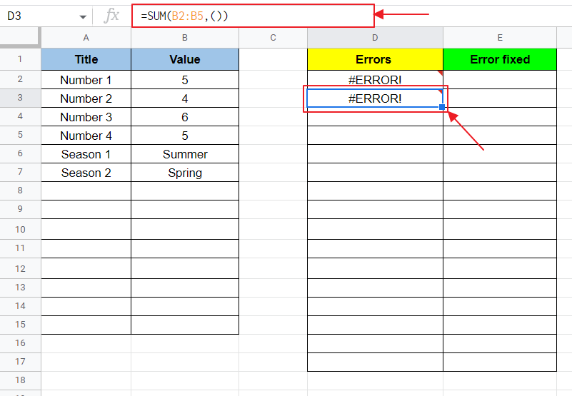
Always remember when you are following the correct syntax in formula but keep the parenthesis empty, it is going to result in #ERROR! Error.

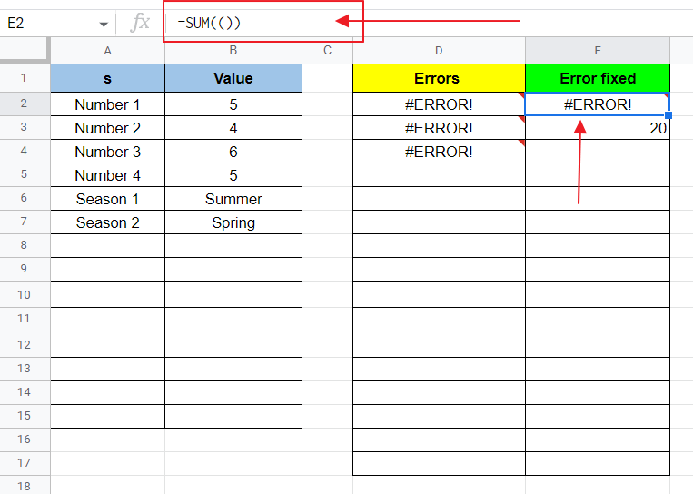
Another example is when you simply give an empty parenthesis to formula as:

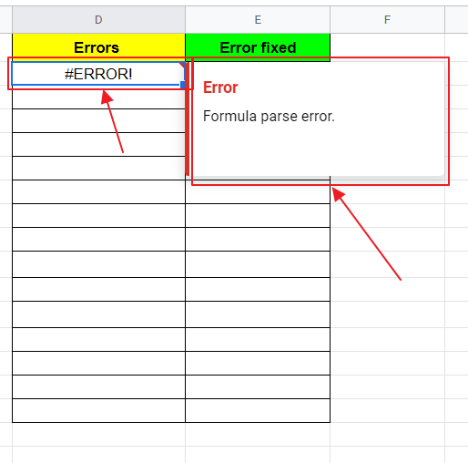
You will get the error as:

We may get this error if we forget to put “,” commas while giving multiple parameters or “:” colon while mentioning the range for a formula as:

And also if closing parenthesis is not applied inside a formula, Google Sheets will automatically insert them if they are missing at the end of formula but if some parenthesis are missing inside a formula, Google Sheets will present the same #ERROR! error.

Now, let us move on how to resolve or fix these #ERROR! Error in Google Sheets.

How to fix #ERROR! Error in Google Sheets?

The way to fix is very simple. All you need to do is to terminate the cause. Since you know that it is empty brackets which is causing Formula Parse Error #ERROR, hence we can either remove those empty brackets or fill them up to avoid empty brackets causing the error.

#ERROR! Fix is:

• Terminate the empty brackets ()
• Fill up the empty brackets ()
• Insert missing comma or colon
• Insert the missing brackets

Method 1: Terminate the empty brackets ()

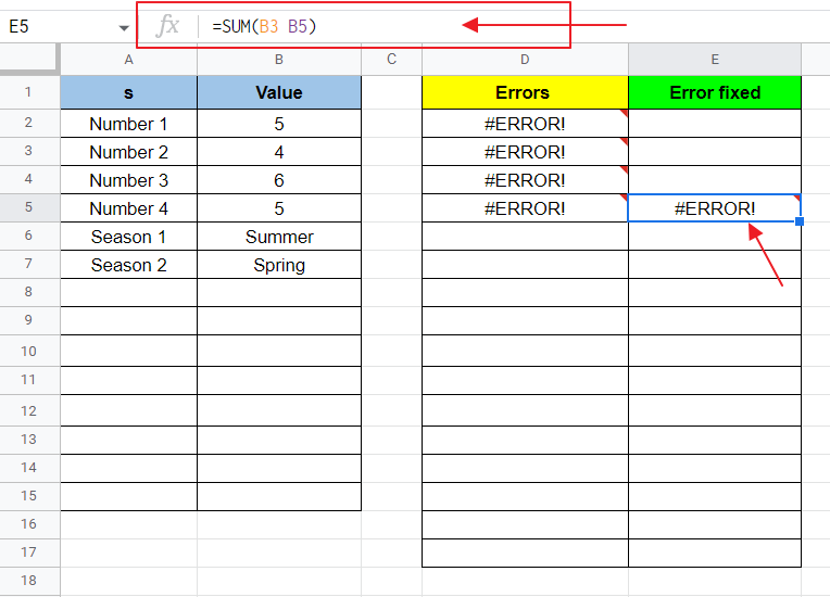
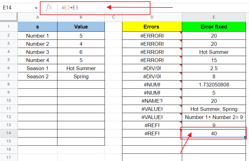
Let us terminate those empty brackets to resolve the error as:

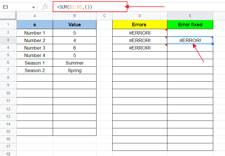
We have #ERROR on the formula “=SUM(B2:B5),())” as below:

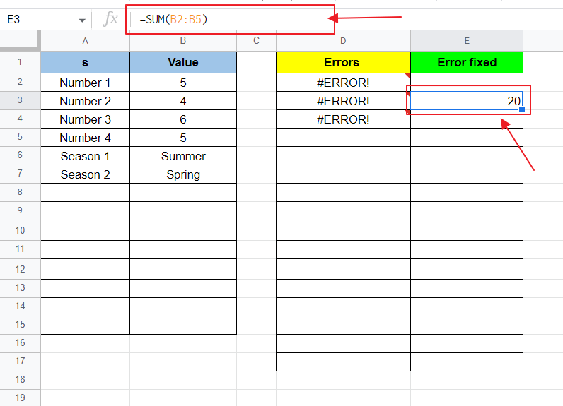
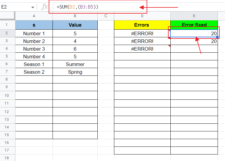
If we simply take out the brackets from the formula, we will get the actual sum between the range of B2 to B5 as:

Now, let try another method to resolve the formula parse error #ERROR!

Method 2: Fill up the empty brackets ()

We can also fill up those empty brackets to resolve the error:

Let us discuss the solution on this error:

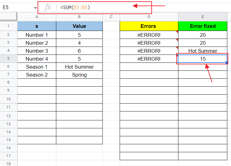
We have this #ERROR! due to empty brackets given as a parameter to the function SUM and there is no other parameter to add up to the value of SUM, so removing such empty brackets would lead to another Formula Parse Error #N/A! (which will be discussed ahead) and defeat the purpose of using SUM function. So, we are in need to add some valid parameter to the SUM function in formula as:

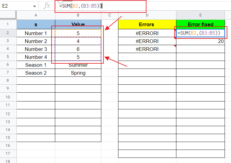
We can fill those empty brackets with any function or value or range that we desire. In above example, the same values Number 1 to Number 4 are added up in SUM as 2 parameters. So we get the same result, sum of Number 1 to Number 4 as:

Now let us take a different approach for filling up the empty brackets giving error as:

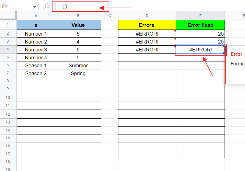
Let us fill those empty brackets to resolve the error as:

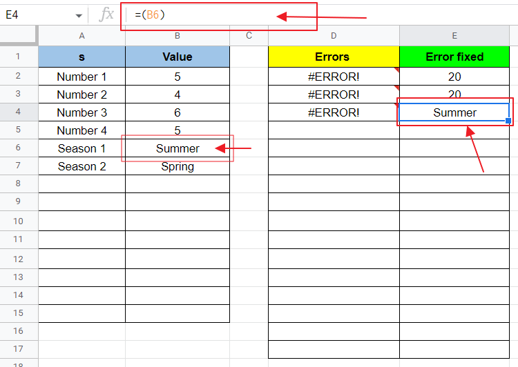
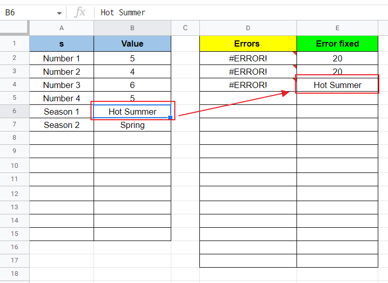
Now, this cell is displaying the value of cell B6, any change in B6 would lead to change in it as well.

Method 3: Insert missing “,” comma or “:” colon

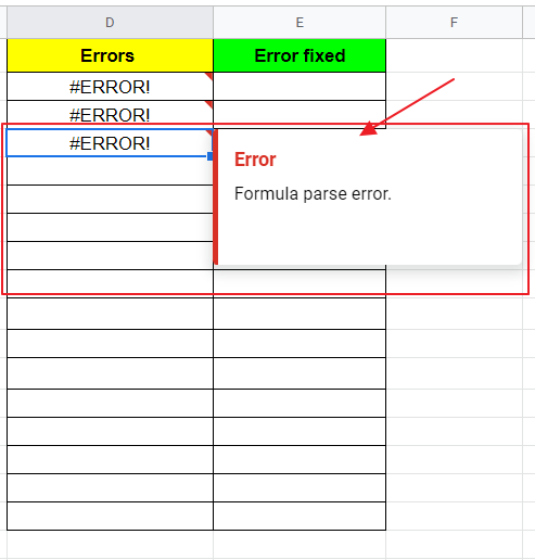
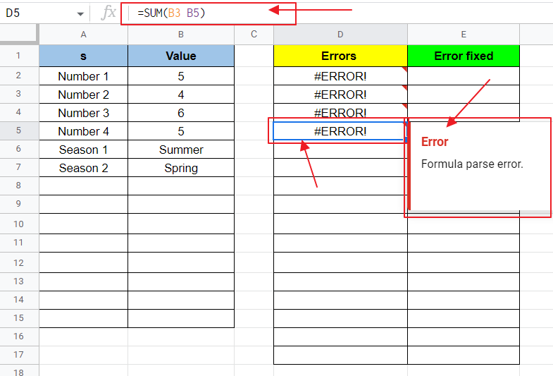
If comma or colon is omitted while giving the parameters to a function, it can also cause #ERROR! error as:

We can insert “,” comma between the two cell names to treat them as 2 separate parameters or insert “:” colon to treat them as a range as:

In this way, using the above methods; we can deal with the Formula Parse Error #ERROR!

Why we get #DIV/0! Error in Google Sheets?

We get Formula Parse Error “#DIV/0!” when we are attempting to divide by 0 in a formula. As dividing a number by zero is an unlimited calculation, resulting in infinity; Google Sheets need not to bother with doing all that calculation and also it is an indication that user is going beyond the required calculations.

We get this error when:

• Formula is directly or indirectly attempting to divide a number by zero in a cell

Let us discuss this error with the help of some examples.

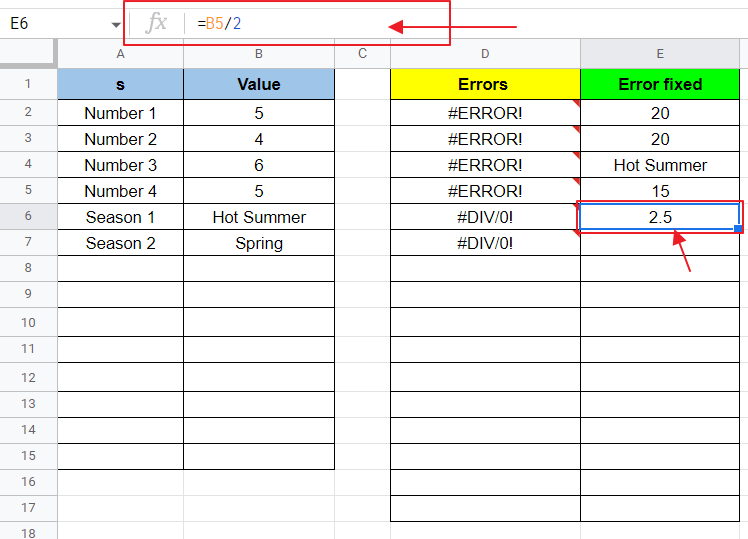
Let us consider the formula:

No matter what the value of B5 is, formula is attempting to divide it by zero resulting in Formula Parse Error as:

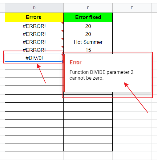
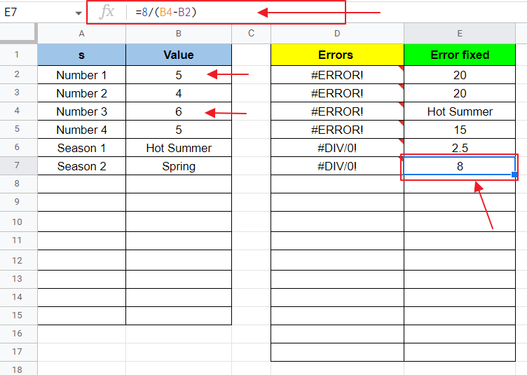
This example describes the intentional or direct dividing by zero. There may be some cases where user is not directly dividing the number by zero but denominator may become zero in calculations as:

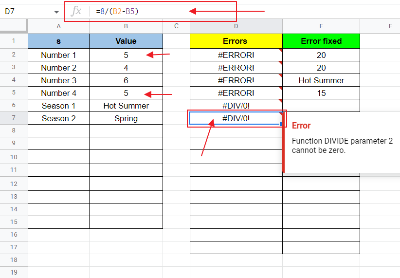
Although the denominator is directly not zero but B2 and B5 have the same value “5” hence their subtraction would lead to zero in denominator and hence #DIV/0! Error.

How to fix #DIV/0! Error in Google Sheets?

One and only way to fix #DIV/0! Formula Parse Error is:

• Make the denominator non-zero

Let us fix this Formula Parse Error #DIV/0! by making the denominator non-zero as:

We have another example for #DIV/0! error when calculations of denominator leads to zero, in order to resolve such a #DIV/0! Error, we must check the denominator part of formula again and make sure that it does not lead the denominator to zero as:

#DIV/0! Errors are easy to resolve as you only need to make the denominator non-zero.

Why we get #NUM! Error in Google Sheets?

We get #NUM! Formula Parse Error when the formula has invalid numeric values.

Common causes of #NUM! error are:

• Formula has an invalid numeric value
• Finding square root of a negative number
• Fetching an invalid number like trying to find 6^th smallest number out of 5 numbers in a range

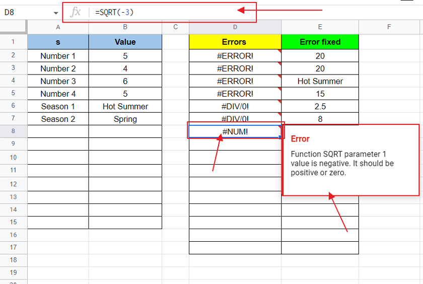
Common example is taking square root of a negative number. Although it is possible to calculate square root of a negative number using imaginary values, it is not possible to calculate it without complex calculations at all. Google Sheets does not entertain imaginary values directly, so it results in an error when you push in a negative values in SQRT function in Google Sheets.

This is what happens when you try to take square root of a negative number using SQRT() function:

Now let us try to find a number that is invalid e.g. 6^th smallest number out of range of 4 numbers. We will still get the #NUM! error as:

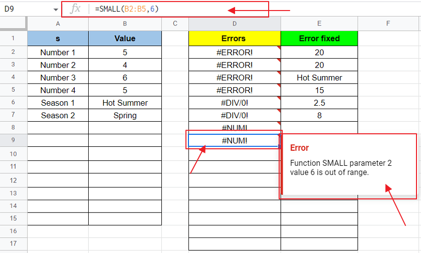
As we are trying to find a number that is not even within the range; we will get a #NUM! Formula Parse Error while trying to use this formula.

Let us move on how to fix this error.

How to fix #NUM! Error in Google Sheets?

When we know the causes, it becomes easy to fix the problem. Here, we discussed the cause of #NUM! error. So, we can fix it easily by eliminating the cause.

You can fix #NUM! Error using the following:

• #NUM! Error occurs due to invalid values, so use only valid values.
• If #NUM! occurs due to attempting to find square root of a negative number, then take positive numbers for taking square roots.
• Do not attempt to fetch invalid numbers like trying to find 6^th smallest number out of 5 numbers in a range; rather fetch valid numbers that exist in a series or range.

Let us fix #NUM! error that occurred due to attempting to take square root of a negative number as discussed above.

We can easily fix this error by taking positive number for taking square roots instead of negative number as:

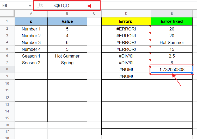
As you can see #NUM! error disappears as we give a positive value to SQRT() function.

We also discussed the occurrence of #NUM! error due to trying to find 6^th smallest number in a range of 4 numbers. In order to eliminate this error, we just need to provide such a position that exists within the range. So, we will just provide a position that exist within the range e.g. find 3^rd smallest number in a range of 4 numbers as:

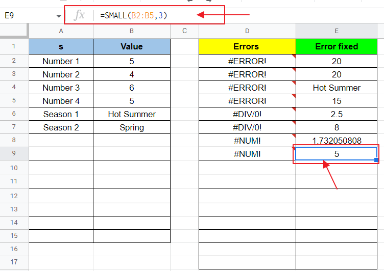
As you can see, in this case, the 3^rd smallest number is shown rather than error.

In this way, #NUM! error is eliminated.

Why we get #NAME? Error in Google Sheets?

We may get #NAME? error when:

• Google Sheets find an invalid name (cell name, range name, etc.) inside a formula.

Let us demonstrate this error with the help of example below:

Let us give name to a range as:

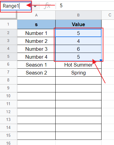
Notice that range name for B2:B5 is “Range1”.

Now let us try to call the range inside a formula using the wrong name as:

Since there is no valid name for cell or range as “Range01” hence it is an invalid name. And so Google Sheet will not recognize this name and hence give a #NAME? Formula Parse Error as:

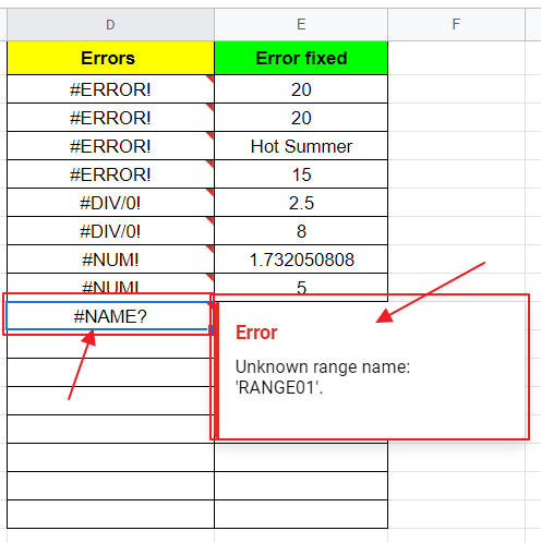
Any invalid name used inside a formula or any function of the formula will cause #NAME? Error as above.

How to fix #NAME? Error in Google Sheets?

#NAME? Formula Parse Error can be fixed by following the instructions as:

• Use only valid names inside formulae (Use correct name after checking spelling mistake in it).

Let us resolve the #NAME? Error discussed above by using the actual valid name of range as:

Now, as the correct name is used inside the formula; #NAME? error naturally gets resolved. And output of the formula appears inside the cell.

Why we get #VALUE! Error in Google Sheets?

#VALUE! Formula Parse Error occurs when formula contains either an invalid value or the value which is not in required format required by the formula.

Common causes of #VALUE! are as:

• Value provided to the formula which are not in correct format. E.g. Adding up an integer and string using “+” operator. In other words, incompatible values inside a formula.
• Unexpected format of values provided to the formula. Example trying to subtract string from another string.

Let us demonstrate the #VALUE! Error with the help of causes discussed above.

Let us write a formula which attempts to add up 2 string values as:

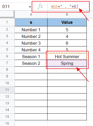
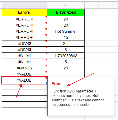
In this example, we want to show “Hot Spring” and “Spring” separated by a comma but we are using the simple “+” operator for the purpose. “+” operator can only be used to add up numeric values and has no way to deal with the non-numeric values and hence Google Sheet show #VALUE! error as:

Let us take another demonstration and try to add up an integer and a string value as:

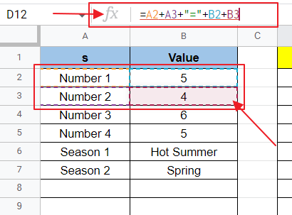
Here, we are trying to show “Number 1 + Number 2 = {SUM(B2:B3)}”. But we are using the simple “+” operator that is used for addition of numeric numbers.

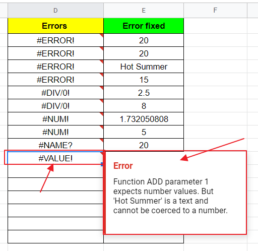
Google Sheets will give us #VALUE! error showing the incompatibility of values inside the formula as:

Any incompatible values inside formula would show up this #VALUE! error as above.

How to fix #VALUE! Error in Google Sheets?

#VALUE! error occurs due to invalid or incompatible combination of values inside a formula; so they can be fixed following the points as:

• Use the correct format of values as specified by the operator or function inside the formula. For example, “+” operator only allows numeric values so use numeric values for this operator.
• Use compatible format of values and the function compatible for them. In order to add the string values from multiple places to a cell, use “CONCATENATION()” function instead of simple “+” operator.

Let us fix the above demonstrated #VALUE! errors.

Let us use CONCATENATION function for adding together 2 or more string values using the formula:

We will get the required result as:

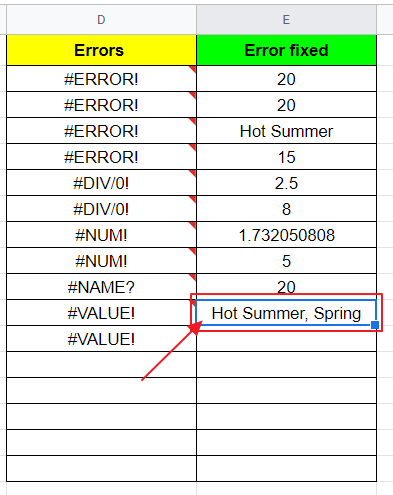
We can see the concatenation of string values i.e. string values being added together as above.

Let us move on to the other example where we need actual sum of two numbers as well as the combination of strings in it.

We will design our formula using CONCATENATION function and use “+” operator inside it to add up the numeric values as:

Using the above formula, we can see a combination of string values followed by the actual sum that took place between 2 numbers as:

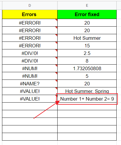
In this way, we can resolve the #VALUE! error and concatenate the string values as well as other sum or subtraction operations alongside inside a single formula as above.

Why we get #REF! Error in Google Sheets?

We may get #REF! error when we attempt to:

• Use a reference of cell(s) inside a formula which does not exist at all. E.g. the reference was deleted.
• Use circular dependency, i.e. reference of the cell containing the formula is also specified within the formula.

Let us demonstrate #REF! Formula Parse Error by using circular dependency as:

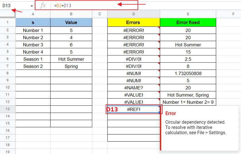
As you see above, the formula is given inside the cell D13 and formula content also include D13 which in turn becomes a circular dependency as above.

Let us take another demonstration into consideration where cell references are deleted after the development of the formula.

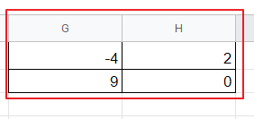
Suppose we have some cells referenced G1:H2 having numerical values as:

Now we develop the formula for their sum as:

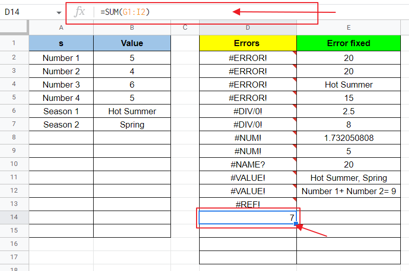
We can see that cell shows the result of formula as reference of the cells given inside SUM is valid.

Now, let us delete those 4 cells. Just as we delete the cells, the reference to those cells become invalid and we will get a #REF! error as:

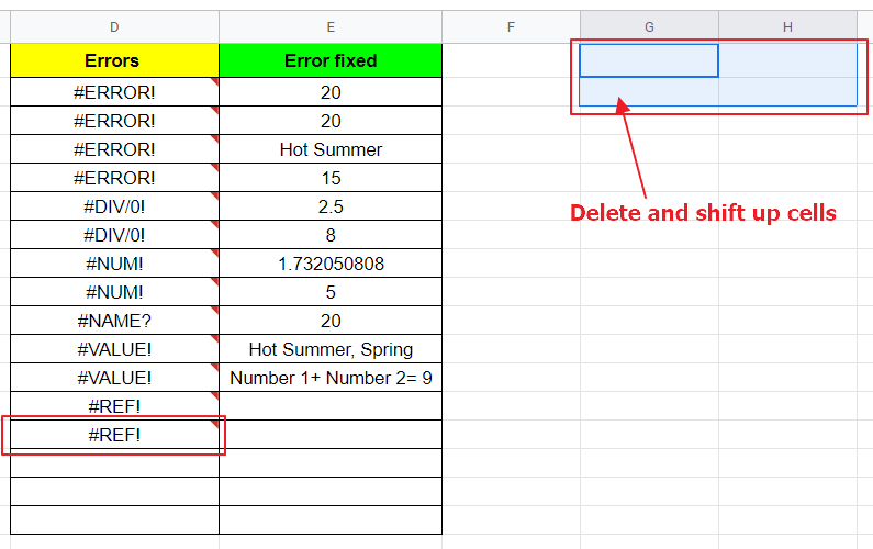
As we can see deleting the cells makes the reference invalid.

How to fix #REF! Error in Google Sheets?

The way to fix #REF! is:

• Provide valid reference to the cells inside any formula.
• Do not delete cells after referencing them inside a formula. And if you move or delete the cells, provide new reference.
• Avoid circular dependency; i.e. do not use reference of the cell containing the formula inside the formula.

Let us fix the #REF! demonstrated above using these methods.

First demonstrated involved circular dependency; let us remove that by avoiding to use the cell’s own reference inside the formula as:

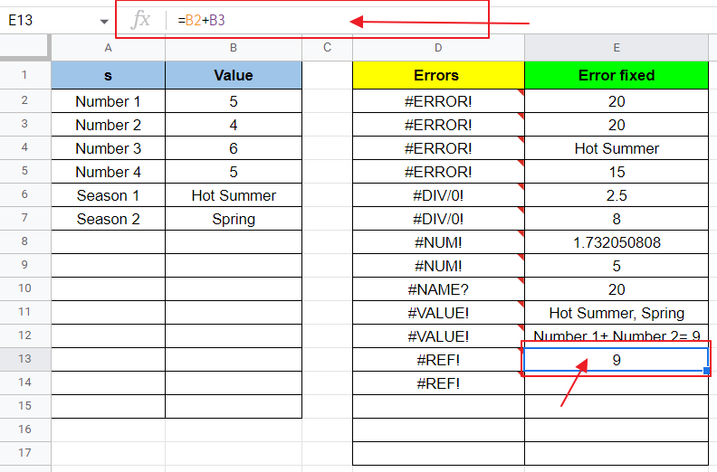
For the other demonstration, let us give a valid reference to the cells as:

#REF! error is very easy to resolve; we only need to provide valid reference of cells inside formula to avoid getting this error.

Why we get #N/A! Error in Google Sheets?

We may get this #N/A! Formula Parse Error when:

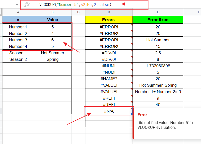
• Google Sheets cannot find what it is looking for. Suppose we are using VLOOKUP function and Google Sheets cannot find any value matching the result.

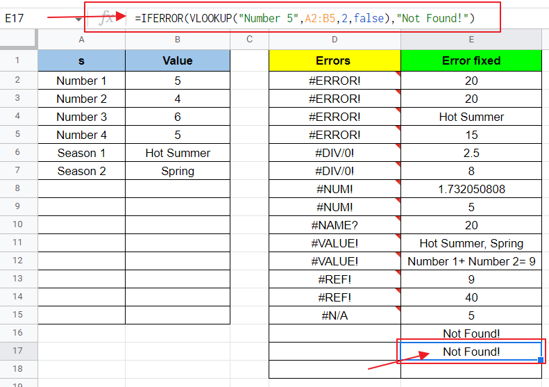
Let us demonstrate this error by trying to look up a value using VLOOKUP function of Google Sheets. Let us find value against “Number 5” (which is not available inside the table) as:

Let us fix this #N/A! error using the following fixing methods.

How to fix #N/A! Error in Google Sheets?

#N/A! error occurs when Google Sheets cannot find what it is looking for and hence has nothing to display. We can fix this error by:

• Only look up the values that exist as to avoid getting this error.
• Use IFNA() or IFERROR() function to display something else in case #N/A! error occurs.

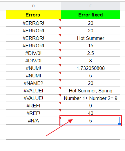
Let us first resolve the error by finding a value which can be looked up in table as:

Here, we are trying to find value right next to “Number 4”. As we know “Number 4” is available in the table can be looked up by VLOOKUP function; so the result is displayed as:

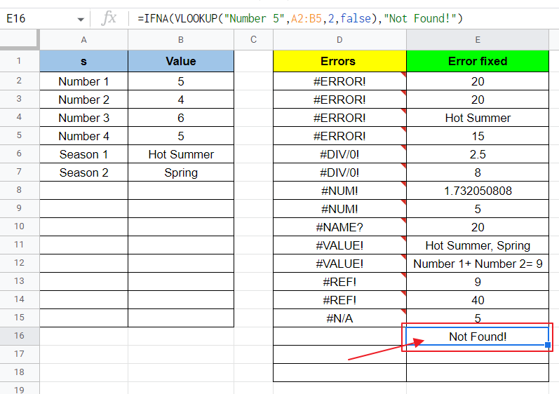
Now, let us fix the same error using IFNA function to display another value if N/A occurs as:

Using this function, if N/A occurs; the cell will display “Not Found!” instead of #N/A! error as:

The same can be done using IFERROR function as:

#N/A! can be fixed using one of the above methods.

Download/Copy Google Sheets Workbook

Important Notes

• We can name a cell, range or table by selecting the cell(s) and writing the name-to-be inside cell name box placed left to formula box as:
• 

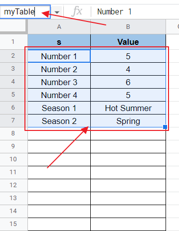
Later this name can be used to specify the range of cells inside any function or formula.

• CONCAT function can be used as an alternative of CONCATENATION function if only 2 strings of text are to be added up together. CONCAT function only takes 2 values as its parameter.
• VLOOKUP function is used to find a value inside a table and show the value next to it or below it according to the index provided inside its parameter.
• IFERROR function would display another value in case any error occurs, while IFNA function is only limited to handle #N/A! error and not the rest of errors.

Frequently Asked Questions

Can I get formula parse error even when I follow the correct syntax of Google Sheets?

Yes, it is possible to get a formula parse error even when you follow the correct syntax of Google Sheets. An example of such error is #ERROR! Error which results when you give an empty parenthesis as parameter to a formula or function. This is explained in detail in the article above along with its fix.

Also, you may get #N/A! error if you are trying to look up a value which is not available. Example is demonstrated above in the article as trying to find the value next to “Number 5” while Number 5 itself is not available in the table.

What happens if you give an empty parenthesis as a parameter to a formula in Google Sheets?

You will get #ERROR! Error whenever you use an empty parenthesis inside any function or formula. It is discussed above in detail.

Why we use VLOOKUP function in Google Sheets?

VLOOKUP function is used to find a specific value and display value next to it or before it according to index number provided inside the VLOOKUP function. If the value to be found is not available in the range provided to the function, then #N/A! error occurs as the value is not available. IFERROR or IFNA function can be used to display another value in case an N/A occurs.

Why we use IFNA function or IFERROR function in Google Sheets?

IFNA function takes 2 arguments, first argument is the value and second argument is the value to be displayed in case #N/A! error occurs inside the value. IFERROR works the same; the only difference is that it can handle all types of errors while IFNA can only handle #N/A! error.

Why we use CONCATENATION function in Google Sheets?

CONCATENATE function is used to concatenate (add together) strings of text. It can take multiple arguments. CONCAT function can be used as an alternative to concatenate 2 strings of text only.

Conclusion

Google Sheets provides us with many functions. Multiple errors may occur while trying to use functions inside formulae of Google Sheets.

Any question about the given topic and methods are most welcome to be entertained. Feel free to share your thoughts in the comment section below.

Thanks for Reading!