How to Use Google Sheets Conditional Formatting Based on Another Column

In this article we will learn about how to use google sheets conditional formatting based on another column.

It is relatively easy to apply conditional formatting based on the current value of the cell. But let’s say you encounter a problem where you have to highlight or format a column based on another column’s values. This type of problems can be solved using google sheets conditional formatting based on another column. In this article, we will discuss how to use google sheets conditional formatting based on another column to highlight or especially format a column based on another column’s values.

Download/Copy Practice Workbook

How to use Google Sheets Conditional Formatting based on another column

If a problem involves to apply conditional formatting based on the value of (same) cell. That’s an easy task. All you have to do is to:

Select the cell -> Apply Conditional Formatting -> Set conditions / rules -> Done

But sometimes you may get across a type of problem where you have to conditionally format a column of cells based on another column’s values. This is relatively difficult task. But don’t worry, this article describes step-by-step easy procedure to apply google sheets conditional formatting based on another column with easy guide and screenshots.

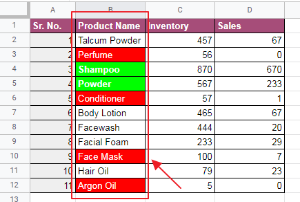
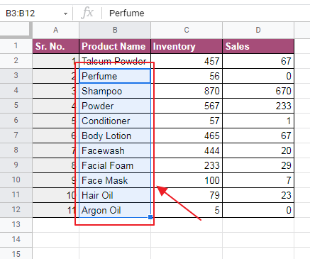
Suppose you have a worksheet containing products and their sales for the past month. Now you have to highlight the product names which had less than 10 sales in red to limit their stock and highlight the products having sales more than 100 to buy more of their stock.

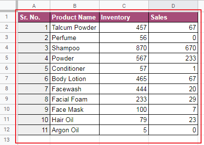
Required format is as:

Generally, there are two methods to achieve this.

1. Apply conditional formatting to range of cells (column)
2. Apply conditional formatting to a single cell and copy it to range of cells (column)

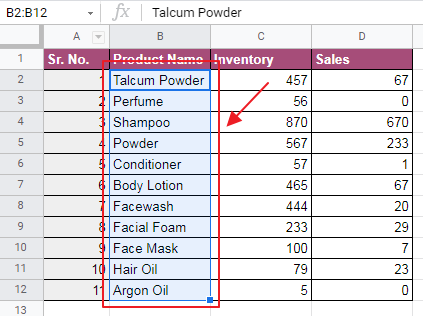
Step 1:

Select the column which needs to be formatted. In this case, select the product name column (excluding the heading). It will highlight in blue as:

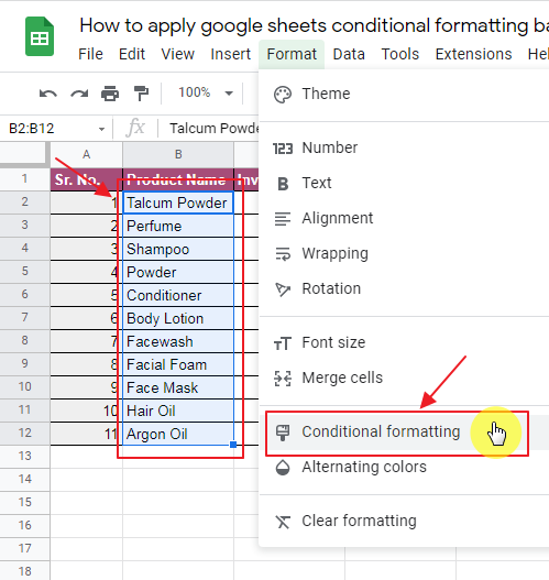
Step 2:

Apply Conditional Formatting either by selecting it from “Format” toolbar as:

OR

Right click the selected column -> Choose “View more cell actions” -> Conditional Formatting

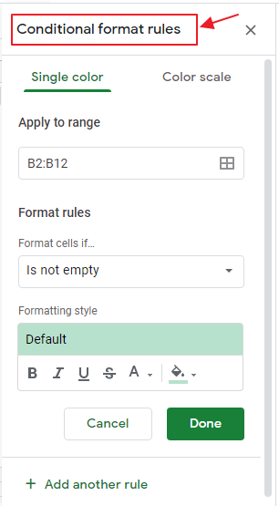
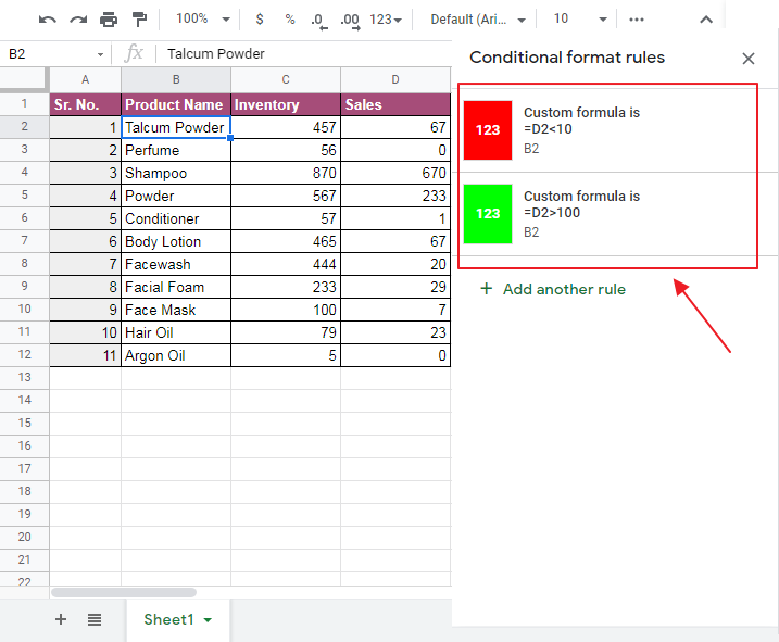
Conditional Formatting Rules Box will appear as:

Remember that we can choose a range of cells by manually typing in the conditional formatting rules box as well. For example, if we choose to Conditionally Format 100 elements of B, we can specify range as “B2:B101”.

Step 3:

Now choose the required Formatting for the range.

select “Single Color” -> In “Format cells if…” column, choose “Custom Formula Is” as:

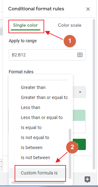
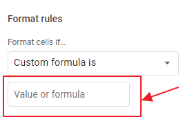
Now in Formatting Rules Section, box will appear for writing formula as:

Step 4:

Write the formula describing the condition for Conditional Formatting.

Here, we need to apply two Conditional Formatting.

• Highlight Products with Sales less than 10 in Red
• Highlight Products with Sales greater than 100 in Green

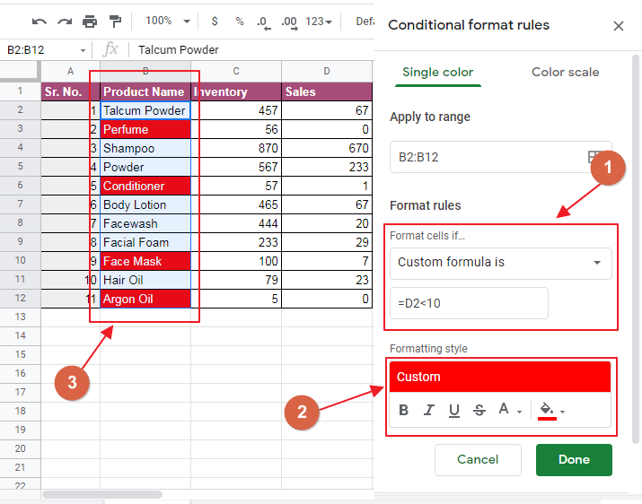
Here, the Formula is that Sales cell corresponding to Product Name cell is less than 10. As Sales lies in D Column and Row number for first cell is 2. So formula becomes “=D2<10” and change the formatting below according to choice (Highlight in red for this case).

You can see side by side that changes are applying to columns as you apply the formula and set the formatting as:

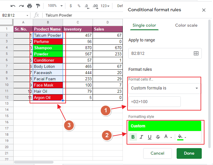
We also need to apply another formatting to highlight in Green if sales are more than hundred, we choose “Add another Rule” below the “Done” as:

Add the next formula “=D2>100” in the same way and apply format of Green Highlight as:

Step 5:

Click “Done”.

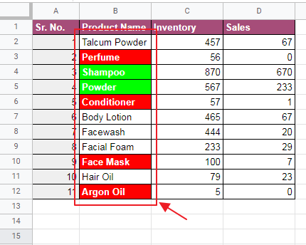
You will see that Formatting have been applied to the required column as:

Step 1:

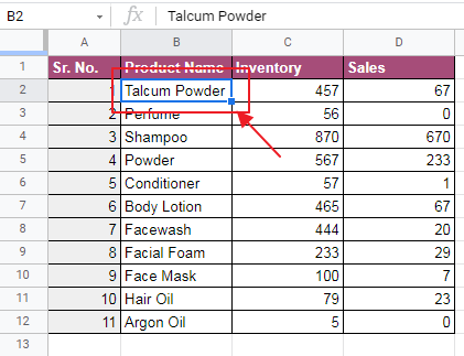
Select a single cell from the column which needs to be formatted.

Here, we will select the first cell as:

Step 2:

Apply Conditional Formatting Rules in the same way (as described earlier)

Right Click -> View More Cell Actions -> Conditional Formatting

Write down the formulae and set formatting rules as:

Step 3:

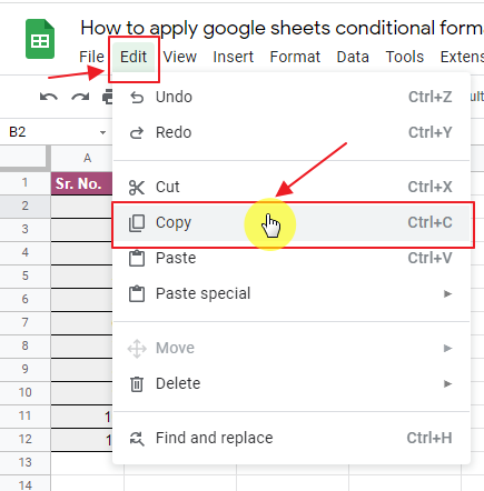
Copy the cell either by

Right Click -> Copy

OR

Ctrl+C

OR

Select “Copy” from “Insert” Toolbar as:

Step 4:

Now select the range of cells (column cells) where you want to apply the formatting.

In this case, we need to apply to column “Product Name” cells. Select them by dragging the mouse over them as:

Step 5:

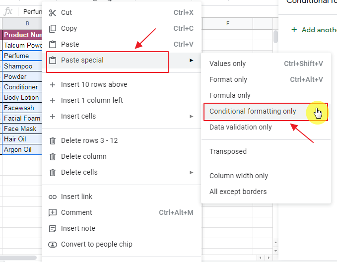
Paste “Conditional Formatting” by:

Right Click -> Paste Special -> Conditional Formatting Only

Now the Conditional Formatting is applied throughout the column.

To know more specific about Google Sheets copy Conditional Formatting, you can refer the article:

How to Copy Conditional Formatting in Google Sheets

Now, we have the final result as:

Notes

If you are using method 2, make sure to remember that any change applied to the cell which was copied will change the rest of the cells of the column where Conditional Formatting was pasted using Paste Special.

Sometimes formula apparently looks correct but does not work properly, some of the major mistakes in applying the formula are:

Excluding “=” when writing the formula:

Some user may forget to put = sign while writing the formula, if so, sheet would not recognize the given condition as formula ad hence no Conditional Formatting will appear although Conditional Formatting is applied.

Cell number might be wrong:

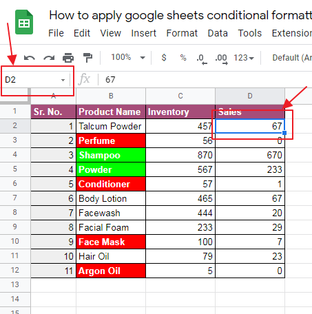
In large worksheets, it is quite difficult to calculate the cell number just by observation so it is better to use a more convenient way.

Click on the cell, whose cell number is required. You can see its number on top left portion of sheets as:

Conclusion

Applying google sheets conditional formatting based on another column provides an easy way to perform Conditional Formatting based on another column values. In this article, easy step-by-step method is described. Any queries are most welcomed. Feel free to comment below for any questions.

Thanks for Reading!