Google Sheets Conditional Formatting If Cell Contains Formula

In this article we will learn about How to Apply Google Sheets Conditional Formatting If Cell Contains Formula by demonstrating a real life problem statement and it solution.

What is Google Sheets Conditional Formatting If Cell Contains Formula?

Conditional Formatting provides an easy way to automatically format the Google Sheets using a formula or condition as and per requirements of the problem. Conditional Formatting also allows us a feature that we can find out and highlight or specially format certain cells if those cells contains a formula. Generally, there are two kinds of cells by the method of inputting value in them.

First is the type where we personally enter the values for them or copy values to them; in either case, they rely on user for their values. Second type of cells are the cells which do not require user to them value; rather they work on an entered formula and fetch values from cells in the formula and process them; the output of that formula is the value displayed in these kinds of cells.

Here, Google Sheets allow us to Apply Google Sheets Conditional Formatting If Cell Contains Formula. In this article, we will provide an easy and step by step procedure to show how to Apply Google Sheets Conditional Formatting If Cell Contains Formula.

Why we use Google Sheets Conditional Formatting If Cell Contains Formula?

Sometimes, while working with Google Sheets, we notice that the value in final output after calculations seem wrong or corrupted. We are mostly dealing with large amounts of data and that data is input very carefully after going through certain checks so we know that it is not the data that is corrupted but our calculations on it.

So, in these types of cases, we might want to highlight the cells which contain a formula in order to check only those cells and minimize time and effort. Google Sheets allows us to use Google Sheets Conditional Formatting If Cell Contains Formula. Using the method for Google Sheets Conditional Formatting If Cell Contains Formula, we can find out those cells which contain a formula and check those cells only to find out the source of problem.

Download/Copy Practice Workbook

How to apply Google Sheets Conditional Formatting If Cell Contains Formula

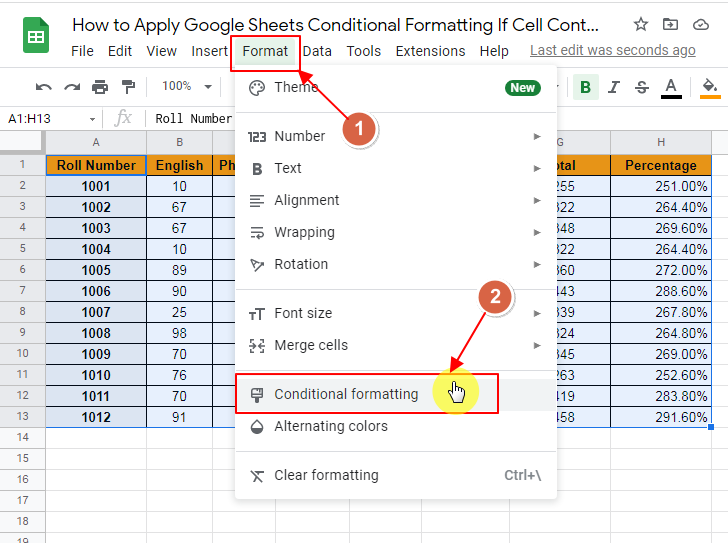
Let us take an example of a Google Sheet where students result is entered and processed. Here, the example contains only a few cells for demonstration. Actually, the data of students may exceed thousands and in that case it will become particularly difficult to find out the cells containing a formula and check those cells. Here we demonstrate the method on the sheet as below:

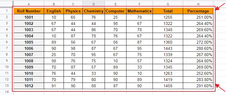
Now, at a careful view, we can see that the student’s percentage exceeds 100% which is not possible by-book. So we need to out the anomaly which is causing the wrong percentage, for that we need to find the cells containing formula; so we can correct them and the sheet can be corrected.

Now, we will apply the method on How to apply Google Sheets Conditional Formatting If Cell Contains Formula.

Step 1:

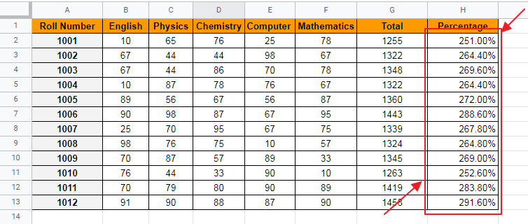
Select the cells where you want to apply the Conditional Formatting.

In this case, we need to apply the Conditional Formatting to the whole table of result to highlight if cell contains formula.

We can select manually by dragging the mouse over the required cells as:

OR

We can type in the range of cells to conditionally format in “Name Box” as below:

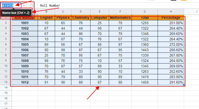
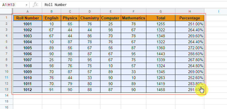
As we select the cells, we see that the selected cells are highlighted in light blue showing selection.

Step 2:

Next step is to apply Conditional Formatting.

As the cells are selected, we can apply conditional formatting using any of the 2 methods below:

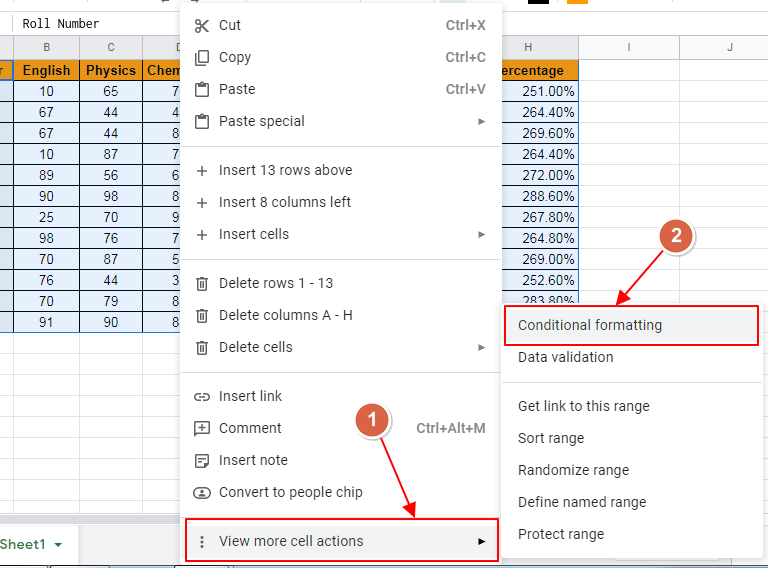
• Method 1: Right Click anywhere on the selected cells. A sub-menu will appear. Choose “View more cell actions” and then Conditional Formatting as shown below:
  • Right Click -> View More Cell Actions -> Conditional Formatting

•  Method 2: From the Format toolbar, choose Conditional Formatting as shown below:
  • Format -> Conditional Formatting

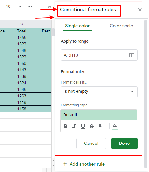
As we click on Conditional Formatting, Conditional Formatting Rules Box will appear as:

Step 3:

Set the condition that is required to activate the conditional formatting.

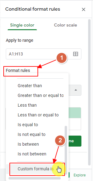
Here, we need to highlight the cells if cell contains formula. So, we apply the condition as a custom formula.

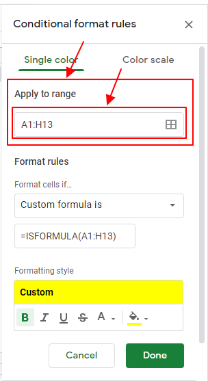
To specify custom formula, select the Custom Formula Is under the Format Rules section as:

Now type down the formula in the Formula or Value Box in Format Rules section. Here the condition is to find out which cells contain formula, so our formula here is “=ISFORMULA(A2:H13)” . We apply it as:

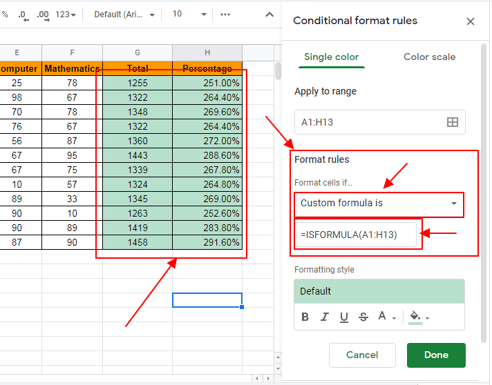
We see that as we apply the formula, we begin to get changes in our sheet.

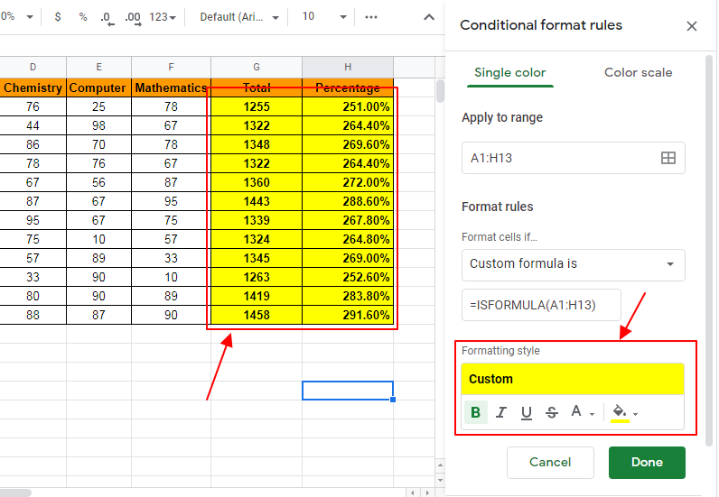
Step 4:

As the condition has been set, now is the time to set the “Format” for Conditional Formatting. We can set our required format in Formatting Style section in Conditional Format Rule Box as:

Step 5:

Click “Done” to specify that conditional formatting has been applied.

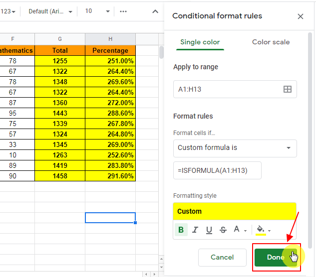
As the conditional formatting has been applied, we can submit it by click Done button or we can also cancel it if we do not require this formatting.

Solution to the problem based on google sheets conditional formatting if cell contains formula

As we get the conditional formatting’s effect on out sheet as:

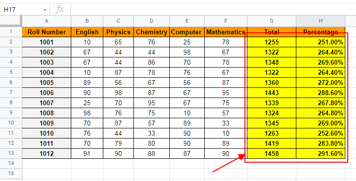
We can easily see that which cells follow a formula or in simple words which cells contain a formula. Now we can check these cells’ formulae to find out where the calculation is going wrong.

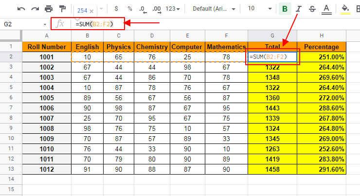
We see that G2 has the formula as:

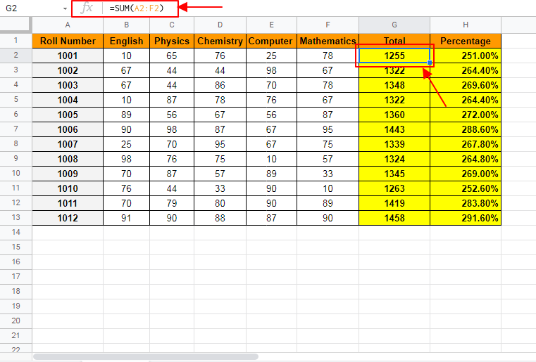
We realize that the formula is also including the value of cell A2 in SUM function which is not required to be added as it is the Roll Number of the student. So, we modify the formula to correct the anomaly as:

As we apply formula to the rest of the cells in Total Column, we get our sheet in correct manner as:

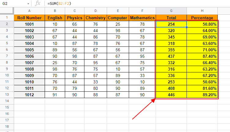
Now we can see the importance of google sheets conditional formatting if cell contains formula. If we checked each cell one by one to check which cells contains formula, it would waste a lot of precious time of user which can be taken to use in an important matter.

Important Notes

We can also set the range of conditional formatting without selecting the cells first and we can also modify the range of Conditional Formatting later after selecting the cells first.

Conditional Format Rule Box appears while showing the range, in its first section Apply to Range, it can be modified by manually typing the required range inside the box as:

Frequently Asked Questions

Can I Apply Conditional Formatting in Google Sheets If a Cell Contains a Checked Box?

Yes, conditional formatting with checked boxes is possible in Google Sheets. By using custom formulas, you can format cells based on the presence of a checked box. This allows you to visualize data or highlight specific information based on the condition you set. Apply this formatting to enhance the usability and readability of your sheets effortlessly.

Conclusion

Applying Google Sheets Conditional Formatting if cell contains formula allows us to find certain cells with formulae in large sheets which enables us to find anomalies in our sheets sooner and save up a lot of time of user. In this article, easy step-by-step method is described. Any queries are most welcomed. Feel free to comment below for any questions.

Thanks for Reading!