How to Use HLOOKUP Function in Google Sheets [User Guide]

Hi, in this article, we will learn how to use the HLOOKUP Function in google sheets.

Many of you have already heard and or used the similar term VLOOKUP in google sheets, but what is HLOOKUP? Is it something like VLOOKUP? Yes, you can say it is the sibling of the VLOOKUP, HLOOKUP, and VLOOKUP both are from the LOOKUP family that is made for search for a key island lookup them in a specified range. VLOOKUP stands for vertical lookup; which means that it looks for the values to be searched in vertical order, and HLOOKUP stands for horizontal lookup; which means that it looks for the values to be searched in horizontal order.

Now VLOOKUP is undoubtedly the most common and most used in google sheets. the reason is the default format of google sheets. Google sheets data is by default set to vertical order, we barely see some data in horizontal order, but it does exist so we need to know to work on it. To perform the same search function on horizontally written data we use HLOOKUP instead of VLOOKUP.

Table of Contents

HLOOKUP Function in Google Sheets

We use large data sets on google sheets and we often need to search the values in the specified range or section in our google sheets file. Normally we use VLOOKUP to search for the key in column-wise format, but we now have data that is written in row-wise order so what we will do? Surely, VLOOKUP will not work on it, so here comes the HLOOKUP, we need to learn how to use HLOOKUP to search the key in a horizontally written dataset. We need to learn how to HLOOKUP in google sheets to search the key_value smoothly in the absence of VLOOKUP, HLOOKUP helps us to perform a search on horizontal data and get the corresponding value.

To perform a key_value search on a vertically aligned dataset
To deal with row-wise data
To use the VLOOKUP functionalities in a transposed manner.

How to Use HLOOKUP Function in Google Sheets

To learn how to use the HLOOKUP function in google sheets, we need some examples to implement and learn the procedure.

I have an example of vertically written data on which I will apply the HLOOKUP formula and we will see how it works.

After that, we will see various use cases of HLOOKUP along with other simple functions.

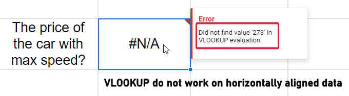
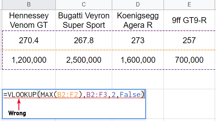
We will also try to use a VLOOKUP on this data so you can understand why we need HLOOKUP, and why VLOOKUP failed for horizontally align data.

How to Use the HLOOKUP Function?

Syntax

=HLOOKUP(search-key, range, index, sorted)

Here,

search-key: is the value to be searched

range: is the range in which we are looking to search the search key

index: is the index number for the row, for which value we want to retrieve against the corresponding search-key value

sorted: is to specify that the data range is sorted or not

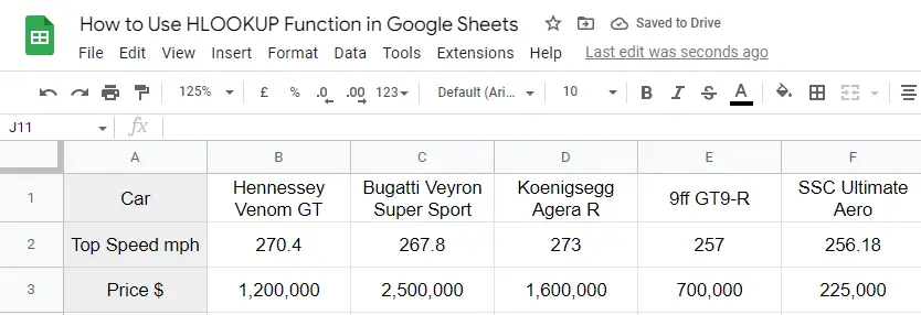
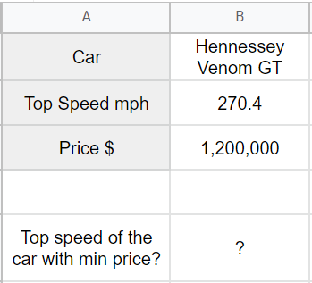
I have a dataset written horizontally, I have top cars, their top speed, and price. We will use HLOOKUP on the data range and see if we can retrieve the corresponding car name by searching for the top speed, or price as the search key. Follow the below step-by-step procedure to understand every detail.

Step 1

Similar sample data to follow the example

Step 2

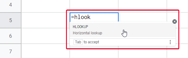
Below is an empty cell start writing the HLOOKUP function starting with an = sign.

Step 3

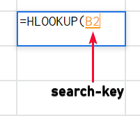
Pass the first parameter (search_key, which we are looking to find in the data range)

Step 4

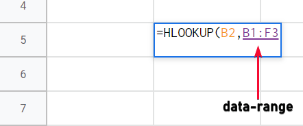
Pass the second parameter (data_range, in which we want to search the search key)

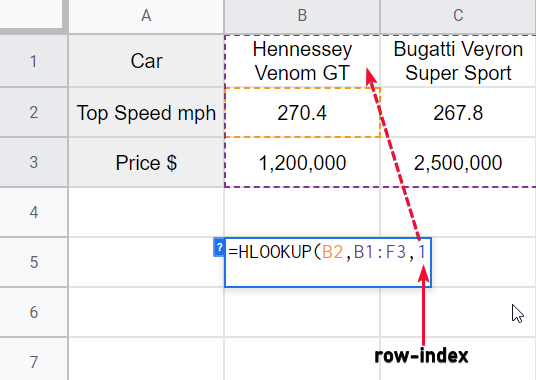
Step 5

Pass the row index (row number from which we want to retrieve the corresponding value of the search key), we provide column index in VLOOKUP as it works column-wise data.

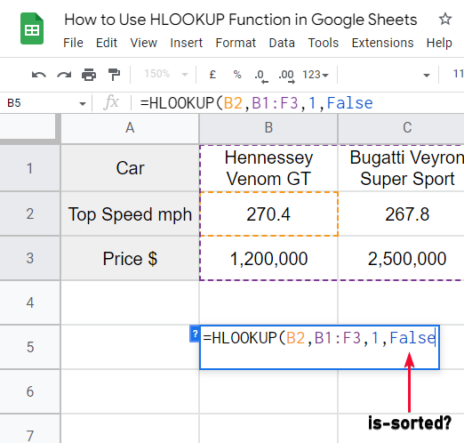
Step 6

Pass False for is_sorted (as we have an unsorted range, pass true if you have a sorted range)

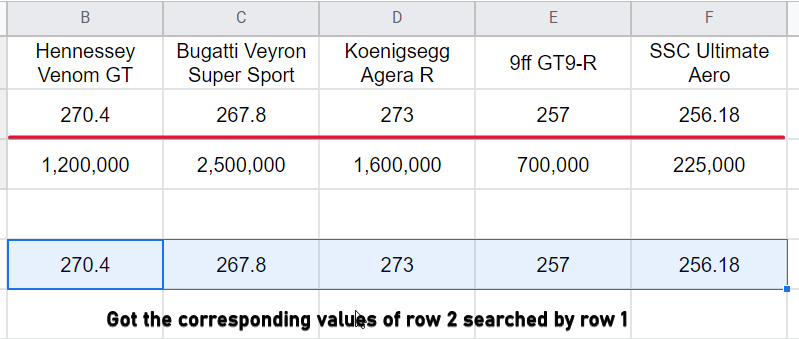
Step 7

The formula is completed, close the final bracket, and hit Enter

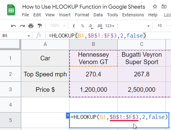
Step 8

Use $ Notation if you want to drag or copy the formula to further columns

This is how to use the HLOOKUP Function in google sheets, below we will see some more variations that can be done using HLOOKUP along with other functions.

How to Use HLOOKUP Function in Google Sheets With Other Functions – HLOOKUP with MIN Function

Syntax

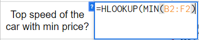
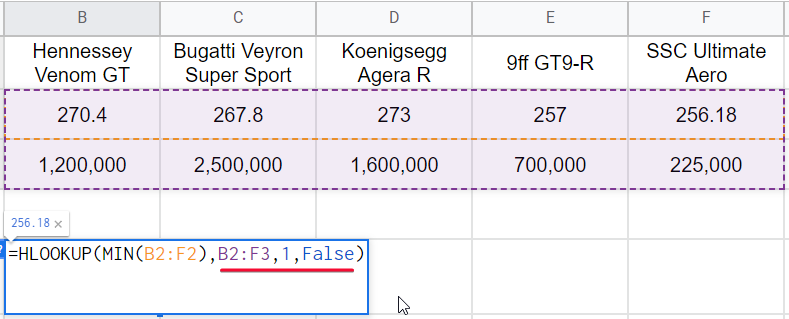
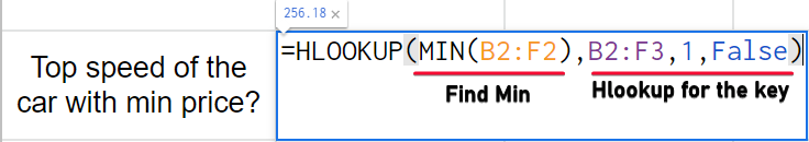
=HLOOKUP(MIN(B2:F2),B2:F3,1,False)

Here,

Min: is the function to find the minimum value

B2:F2: is the range in which we want to get the min value

B2:F3: is the range in which we want to search for the value

1: is the row number relative to the formula

False: is-sorted? false for unsorted range

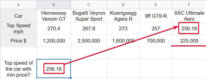
We have the same data set but this time we have to find the top speed of the car that has the minimum price. This is how we can use this formula

Step 1

Find the top speed of the car with the minimum price.

Step 2

Adding MIN function

Step 3

Pass the arguments for HLOOKUP Function

Step 4

Final Formula

Step 5

The result

How to Use HLOOKUP Function in Google Sheets With Other Functions – HLOOKUP with MAX Function

Syntax

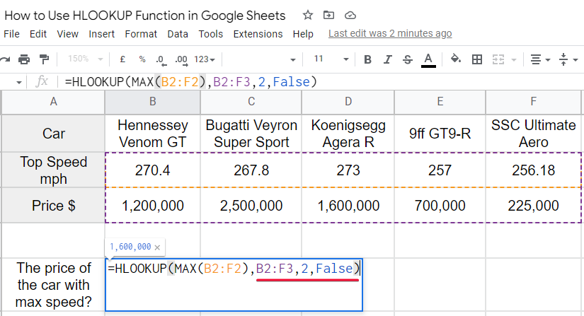
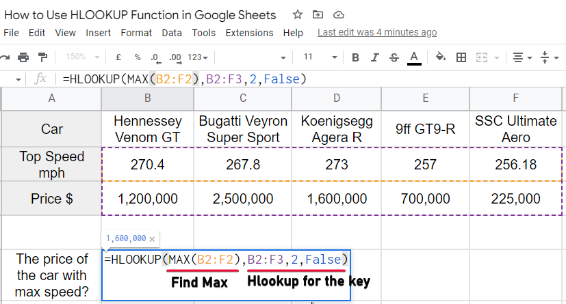
=HLOOKUP(MAX(B2:F2),B2:F3,2,False)

Here,

Max: is the function to find the maximum value

B2:F2: is the range in which we want to get the max value

B2:F3: is the range in which we want to search for the value

2: is the row number relative to the formula

False: is-sorted? false for unsorted range.

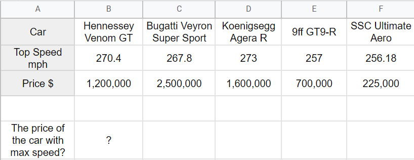
Step 1

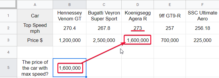
Find the price of the car with the max speed.

Step 2

Adding MAX function

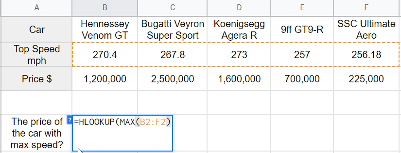
Step 3

Pass the arguments for HLOOKUP Function and you have got the result

Step 4

Final Formula

Step 5

The result

How to Use HLOOKUP Function in Google Sheets – Difference between VLOOKUP and HLOOKUP

VLOOKUP and HLOOKUP are from the same LOOKUP family, VLOOKP is for vertical looking up the data, and HLOOKUP is for the horizontal lookup of data. We use VLOOKUP for the data that is aligned column-wise and we use HLOOKUP for the data that is aligned horizontally. This is the only difference, in syntax, we have no difference both works the same just with a difference in data orientation.

Cons of the HLOOKUP Function in Google Sheets

Two common problems with the HLOOKUP function

For search_key, HLOOKUP always uses the first row only within the given range. So it is not possible with the HLOOKUP Function to retrieve a value that is above this row.
HLOOKUP function does not have the power to auto-update itself when some changes are made to rows, such as inserting a row or two between the specified cell range, it will not automatically update the row index, we have to update it manually inside the formula.

Important Notes

HLOOKUP functions are very powerful and can be used along with many formulas and functions.
HLOOKUP can be named as a transposed VLOOKUP function
We cannot get the custom row value against a search key other than the first row we selected as the entire range
HLOOKUP, as well as VLOOKUP, are not powerful enough to auto-update the live changes, if a row is added or removed, or a column is added or removed, they cannot auto-detect and update themselves, we have to manually change the data range as per the new rows.
Remember that the last argument (is-sorted), is important when you are working on sorted ranges. You can easily get the sorted data if you tell the formula that you have a sorted list.

Frequently Asked Questions

How to use VLOOKUP in google sheets?

We have discussed, how to use the HLOOKUP Function in google sheets in the very first section. To use the VLOOKUP function in google sheets you should have horizontally aligned data and you can use the formula directly on it similarly to VLOOKUP, if you have any problems, please refer to the above section where I discussed everything in detail with screenshots of practical implementation.

Is the Transpose Function in Google Sheets Similar to the HLOOKUP Function?

The transpose function in google sheets is not similar to the HLOOKUP function. While the transpose function allows you to switch the orientation of a range of cells, the HLOOKUP function is used to search for a value in the top row of a range and retrieve a corresponding value from another row.

What is the difference between HLOOKUP and VLOOKUP?

The only difference between HLOOKUP and VLOOKUP is the orientation of the data, you may have a google sheet file in which you have multiple data tables, some can be vertically aligned and some can be horizontally aligned you can do the same for both of these data using VLOOKUP for vertically aligned data, and HLOOKUP for horizontally aligned data. There is no syntactical difference.

How to retrieve the corresponding value using VLOOKUP?

We can define the row index, as we define the column index in VLOOKUP, here we have the row index in HLOOKUP. The third argument is to define what to retrieve corresponding to the searched value. Here you can pass row indexes such as 1,2,3. Remember that they are not the actual row number, they are indexed within the context of the HLOOKUP formula for example if your data is in rows 1-10 and you have applied the formula on the range from rows 3-5, so your indexing will be 1 for row 3, 2 for row 4, and 3 for row 5.

Conclusion

Wrapping up how to use the HLOOKUP Function in Google Sheets, we have learned step by step about the uses of this function and how it is different from the VLOOUP function, we saw why we need to learn how to use HLOOKUP in google sheets. Then we learned the complete method to practically implement the HLOOKUP function on horizontally aligned data, then we made some combinations, and we saw how to use the HLOOKUP function with MIN Function, and MAX Function. We saw the difference between VLOOKUP and HLOOKUP and this is how you can do it. You can become the master of HLOOKUP by following this article with step-by-step implementation.

That’s from How to use HLOOKUP Function in Google Sheets, see you soon with another helping tutorial, till then take care. Don’t forget to like share and subscribe to our Blog. Thank you. Keep learning with Office Demy.