How to Format Cells in Google Sheets [Guide 2023]

Google Sheets is a spreadsheet software from Google that has tabular pages with small cells all over the page. When we use Sheets, we write our content within cells, and to format the content, we need to know how to format cells in Google Sheets. In this article, we will learn how to format cells in Google Sheets. We will learn all the formatting options and will practically implement them to make use of all the features Google Sheets is providing for free.

We have many features that lie under a different section of the cell formatting. Some features are about text and some for cells body and background. I am not including cell size in this guide since it’s a different thing, and we will only be focusing on cell formatting.

Importance of Formatting Cells in Google Sheets

Where everything is inside the cell,  we have no other option to format the document, but to format the cells. We can format the cell’s body, size, color, and so many things. This is the only way a sheets file can be decorated, formatted, designed, or customized. So, learning how to format cells become very significant.

This article is fully focused on formatting cells. We can format the text inside the cells using cell formatting, we can control the size, font type, bold italic, and so many things within the cell. We have so much to learn today, most things are very common and you must be already using them in your day-to-day tasks, but for absolute beginners, this guide is going to be complete and concise. So, let’s get started.

How to Format Cells in Google Sheets?

I have planned to break down this entire topic into smaller chunks, so you can skip it if you know a specific thing already. I will cover different types of formatting in different sections from basic to advanced. Let’s start with the basic formatting options we have.

How to Format Cells in Google Sheets – Format Text inside Cell

In this section, we will learn how to format cells in Google Sheets, and specifically, we will see how to format text inside the cell. Formatting text inside the cell is all about making content more attractive, we make format changes to decide how our content looks, so in this section, let’s see what features Google Sheets have to format our text inside the cell.

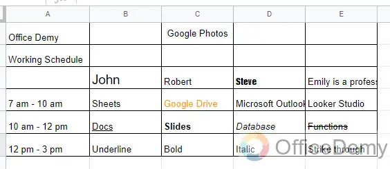
Firstly, you should have a demo file to make these changes practically. I have some sample data, and I will use this file in this entire tutorial.

Change the Font Size

We can change the font size of the text inside the cell. There are so many numbered values available for it, we can also type a number to get the corresponding font size.

Note: Changing font size does not change the cell size.

Step 1

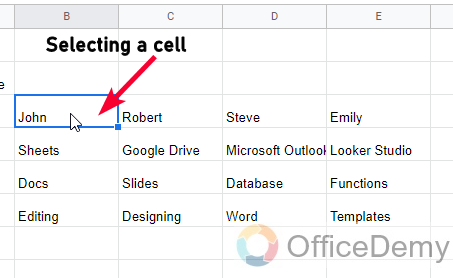
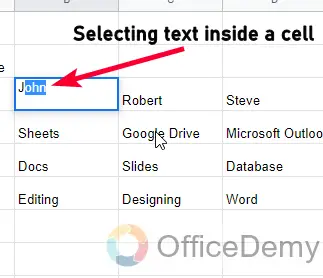
Select the cell or the text inside the cell by mouse selection.

Step 2

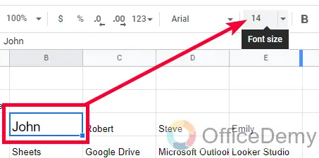
Go to the Font size dropdown, and pick a value from so many numeric values

Step 3

Your font size is changed successfully!

Change the Font Family

We can change the font family for the selected font, there are so many font styles available in Google Sheets, and you can also get more fonts from add fonts options.

Step 1

Select the text inside the cell, or select the entire cell(s)

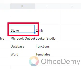
Step 2

Go to the Font dropdown in the toolbar, and select from the so many available font Families.

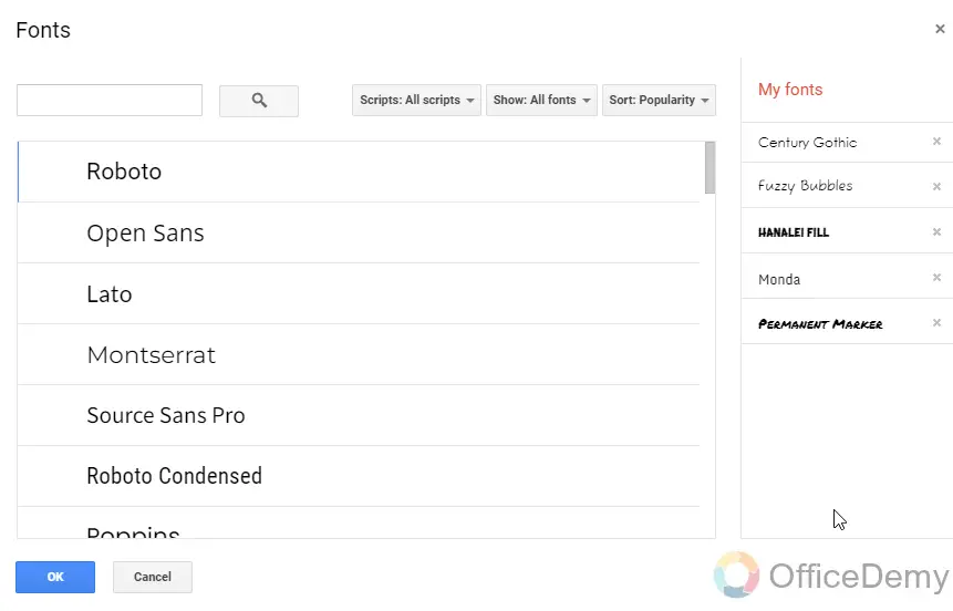
Step 3

Click on the More Fonts button to get more fonts.

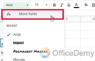
Step 4

You can see your font family for the selected cell(s) is changed.

Change the Text Color

We can change the color of the text for the selected cell or text. There is almost every color available in the color box for font or text.

Step 1

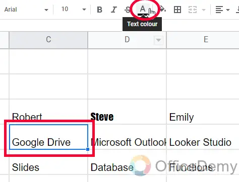
Select the entire cell or a part of the text inside it

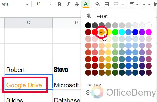
Go to the A symbol in the toolbar, its font color, and select a color.

Step 2

You can see your text color is changed to a newly selected color.

Make text Bold Italic Underline or Strikethrough

You can style your text with these three basic formatting types.

For using any of these, the first step is to select the text

Step 1

Select entire cells, or select a specific part of the text inside cells

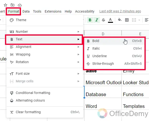
In the toolbar, you can see B (it’s a bold button), I (it’s for italic), and an S (It’s for strike through) but there is no shortcut button for underlining in the toolbar.

Step 2

You can go to Format > Text > Here you have Bold, Italic, and Underline. Click on any of these to apply this style to your selected cells.

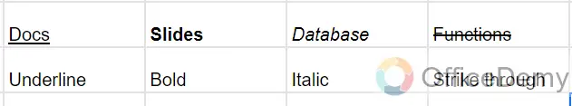
Step 3

Here, you can see the result.

Keyboard Shortcuts

• Bold = Ctrl + B
• Italic = Ctrl + I
• Underline = Ctrl + U
• Strikethrough = Alt + Shift + 5

Step 4

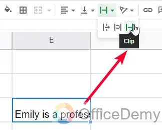
You can also use text wrapping. There are three types of text-fitting options.

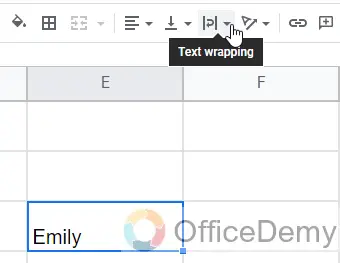
We can use

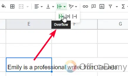
Overflow: It will make the text-overflow outside the cell

Wrap: It will wrap the text and move to a new line; this will automatically increase your cell height.

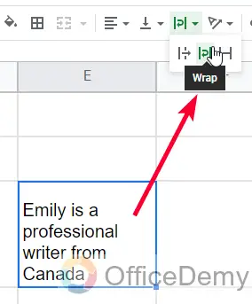
Clip: It will clip the text from both sides, and will only show the partial text depending on the space inside the cell.

How to Format Cells in Google Sheets – Text Alignment

In this section, we will learn how to format cells in Google Sheets and we will see everything about the text alignment. In Google Sheets, we have both alignments options, vertical-align, and horizontal-align. Let’s see how we can use these features.

Step 1

This is a sample text written with default formatting.

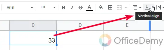
Step 2

To align this text center vertically. First, select the cell or text, then go to the button Vertical align in the Toolbar

Step 3

Click on it, and you will three options. You can select Top, Middle, or Bottom to align your text accordingly.

This is how you can align your text vertically.

Step 4

The same method for horizontal alignment, only the button is different. Left to it, you have another button that can be used like this to align your text horizontally. Three options are here which are Right, Center, and Left.

How to Format Cells in Google Sheets – Fill Color & Border

In this section, we will learn how to format cells in Google Sheets, and we will see how to use fill color and border. The fill color is the cell color, and the border is the cell border that can be on a single border or an entire range. There are many types of borders and we can use the colored border as well with different line styles.

Step 1

To apply fill color on a cell, or a group of cells, select the cell(s) and then go to the Color bucket icon in the toolbar. It’s a fill color feature.

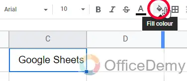
Step 2

Now you can select any color, and it will be added as a fill color or background color of the cell(s)

Step 3

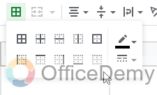
To apply a border on a cell, first, select the cell or an entire range

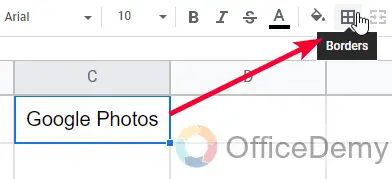
Step 4

Go to the border icon in the toolbar, and here you have so many types of the border, click on anyone to apply to the selected cell(s).

Step 5

Your borders are successfully applied.

How to Format Cells in Google Sheets – Data Types

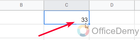
In this section, we will learn how to format cells in Google Sheets and how to configure data types. We have some default formatting for the data types such as numbers always floating to the right side, similarly. The text is always floating on the left side.

If you have written anything in the cell, then it will automatically take the formatting for that specific data type. Now if you remove that and add any other data type then the format will not be changed, and you will need to change the format manually.

Step 1

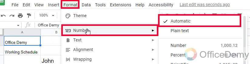
A cell with some text written in it

Go to Format > Number, and you will see the Automatic option will be enabled. This means this is an automatic format taken by Google Sheets based on the data type.

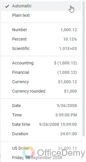
Step 2

To change the data type, go to Format > Number, and here you can the data types from the given list.

There are so many options to format your text accordingly.

Important Notes

Frequently Asked Questions

How do underline cells in Google Sheets?

You can apply only the bottom border to a cell to make it look like an underline effect, else you can use the native underline feature from the toolbar. The keyboard shortcut for underlining is Ctrl + U

Are Borders a Part of Cell Formatting in Google Sheets?

Yes, formatting borders in google sheets is a crucial part of cell styling. By adding and customizing borders, you can enhance the visual appeal and organization of your spreadsheet. Whether you want to create a grid-like structure or highlight specific cells, mastering the art of formatting borders in Google Sheets will take your data presentation to the next level.

How to write subscripts and superscripts in Google Sheets?

Unfortunately, there are no direct shortcut buttons for superscripts and subscripts in Google Sheets. Nor we have these features inside the Format menu. But there are some workarounds you can do. But They do not come under the scope of cell formatting, you can find the complete superscript and subscript tutorial here.

Conclusion

This was all about how to format cells in Google Sheets. We have learned all the cell formatting tools and features breakdown in different sections. I hope I have covered all the important things, and all the formatting options and features that can be used in normal day-to-day tasks. I am closing this tutorial here hoping I have cleared all the key points and useful features inside the scope of cell formatting in Google Sheets. I will see you soon with another useful guide, till then take care. Keep learning Microsoft 365 and Google Workspace with Office Demy.