
To format phone numbers in Google Sheets:
- Select the cell or cells with unformatted phone numbers
- Navigate to “Format” in the menu > Choose “Number” and then “Custom number format“
- In the custom number format box, enter the desired format using placeholders and symbols (e.g., “(###) ###-####” for US numbers)
- Click “Apply“
To write custom number formats in Google Sheets:
- Determine the format you want, e.g., US domestic, US international, etc
- Create the format using placeholders and symbols, like “#” for digits, “-” for dashes, and “+” for international codes
- Manually format your phone numbers according to your custom rules.
Formula Techniques:
- Understand the numbers in the phone number format; “#” represents a digit.
- Comprehend the characters used in phone number formatting, like parentheses, dashes, and spaces.
- Use the formula =VALUE(REGEXREPLACE(A1,”[^[:digit:]]”, “”)) to remove existing formatting.
In this guide, we will learn how to format phone numbers in Google Sheets. Only with a little know-how and minimal effort, you can easily learn how to format phone numbers in Google Sheets, any way you’d like them to appear. So, in this article, I will show you three ways to format phone numbers in Google Sheets, we will also learn how to change the phone numbers from different countries’ formats.
Although, there is no pre-defined method to do it, with some tricks and some handy workarounds we will do it very easily. For this tutorial, we’ll be using standard United States phone numbers, and then I will show you how to format them as other phone numbers, so this tutorial is going to be very fun and full of learning.
Importance of Formatting Phone Numbers in Google Sheets?
When we are working with data, we most probably have the phone numbers in our data, and it’s difficult to maintain phone numbers with correct formats because the numbers may be of different number formats, there can be fewer or more numbers in a complete phone number of a different territory. So, to manage all these things, it’s better to learn ways to format phone numbers in Google Sheets.
Fortunately, we can make a custom format in Google Sheets, and just like numbers, dates, currency, times, and many other formats we can also make a custom phone number using them, there are some other methods as well. We will see all of them, so these are the reasons we should learn how to format phone numbers in Google Sheets.
How to Format Phone Numbers in Google Sheets
There are three primary parts in which we can divide this topic to learn it completely. There are formulas included when we work with numbers, so from this section, let’s categorize the sub-parts and learn each in a single section. Let’s get started with how to format phone numbers in Google Sheets using custom formats.
Format Phone Numbers in Google Sheets – Using Custom Formats
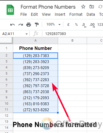
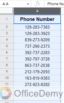
In this section, we will learn how to format phone numbers in Google Sheets using custom formats. We can make any format as per any country’s phone number very easily. I have sample data here in which I have phone numbers in plain format means “unformatted numbers“. We will see how we can change them into a US-based phone number very easily.
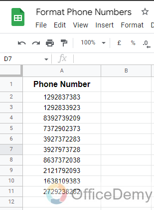
Step 1
Sample data with phone numbers unformatted.
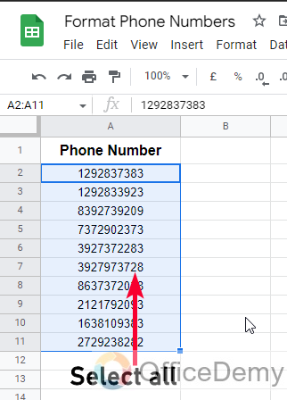
Step 2
To format all the numbers, simply select all the numbers in the column.
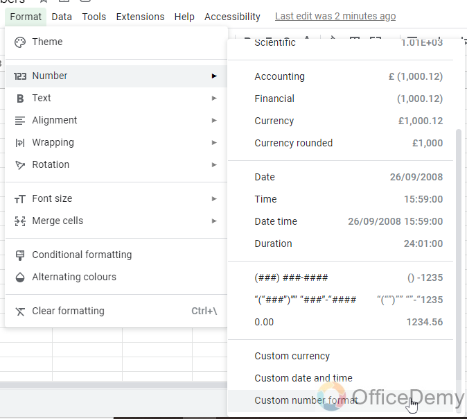
Step 3
Go to Format > Number > Custom number format.
Step 4
In the search box inside the custom number format write the format for a US phone number like below
(###) ###-####
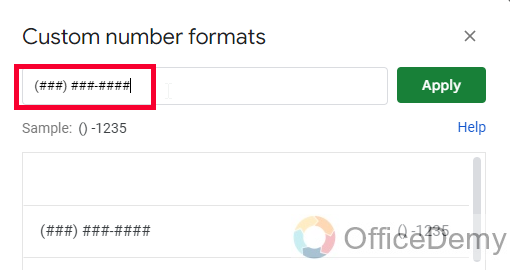
Step 5
Click on the apply button.
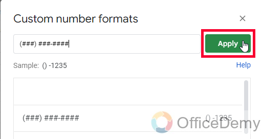
Here, the brackets remain the same, and the dash will also remain the same, only hashes will replace the original numbers.
if you have some other characters in your required phone number format then you also use dots, periods, hyphens, plus signs, and so on.
Using this rule, you can any number format in the world.
Format Phone Numbers in Google Sheets – Write Custom Phone Number Formats
In this section, we will learn how to format phone numbers in Google Sheets, and I will show you how you can write custom phone number formats inside Google Sheets using a simple rule. Below I have some example formats for you.
Here are some common examples of making custom phone numbers in the US.
Step 1
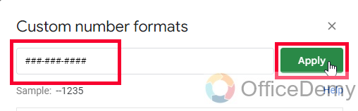
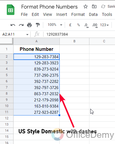
Generating US Style Domestic with dashes: ###”-“###”-“#### = 123-456-7890
Step 2
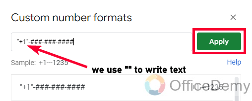
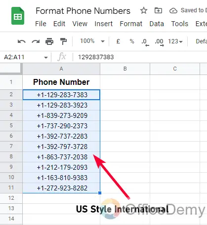
Generating US Style International: “+1-”###”-“###”-“#### = +1-123-456-7890
Step 3
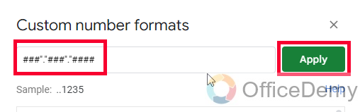
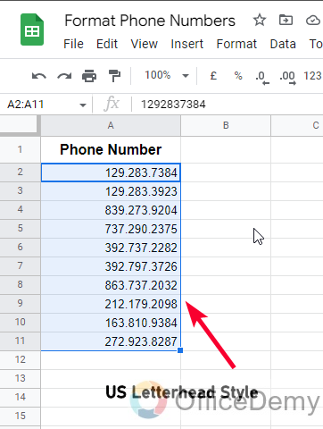
Generating US Letterhead Style: ###”.”###”.”#### = 123.456.7890
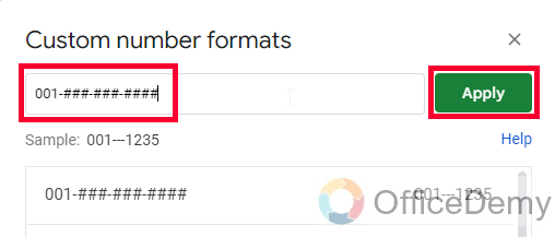
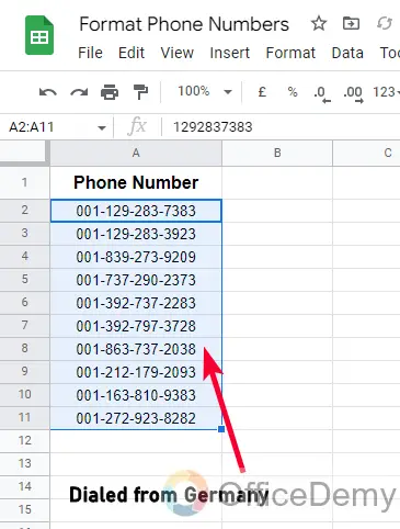
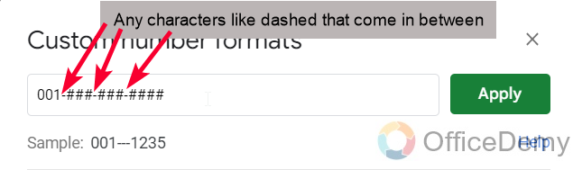
Step 4
Generating Dialed from Germany: “001-”###”-“###”-“#### = 001-123-456-7890
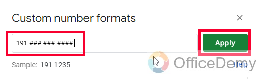
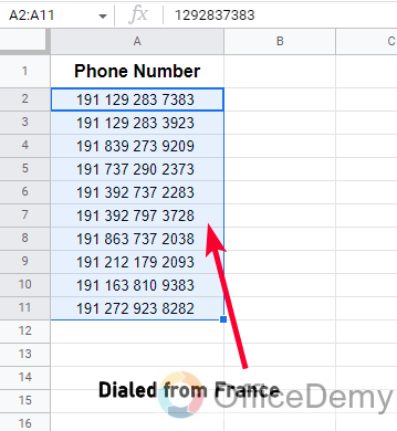
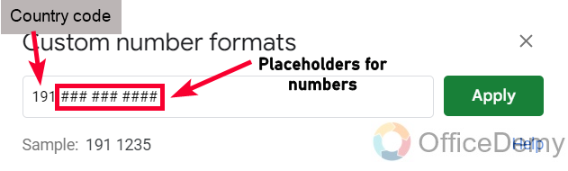
Step 5
Generating Dialed from France: “191 “”###” “###” “#### = 191 123 456 7890
Similarly knowing the pattern of the phone number, you can create any format and then apply it to your plan phone numbers written in Google Sheets
Use corresponding hash codes for numbers and characters as they are, also not that don’t use double quotes when applying for a format in Google Sheets. I hope it’s clear to everyone.
Format Phone Numbers in Google Sheets – Formula Techniques
To make a custom formula we only need to understand two things, one is hash, second is characters. And then we can easily create any custom format for the phone numbers inside Google Sheets. So, in this section, we will learn how to understand the pattern and the formula behind any phone number format. For this, we have to understand some basics. So, let’s get started with some concepts.
It’s very helpful for users that phone numbers are straight forwards, we only have some specific spaces, dashes, points, and other special characters between them, and Google Sheets format creator identity all of them, so it becomes very easy and simple to make any custom format using them.
Step 1
Understand the numbers
The format formula system uses “#” to identify a digit/number, The first “#” value references the first digit, the second “#” identifies the second digit, and so on, we can always have any characters between them they will not break the overall syntax of the formula format.
Step 2
Understand the characters
Depending on the format, we are required to combine parenthesis, dashes, spaces, prefixes, and other textual information with the hashes, they are normally called characters to complete a phone number format, if we skip characters then there will be nothing in our format except the plain numbers with few spaces if we have added.
In Google Sheets, we have to add double quotes to add information between numbers.
Example character keys:
- # = represents the next digit in order of appearance.
- “” = display text
- “ “ = add a space
- “(“ and “)” = display parentheses
- “-” = add a dash
- “.” = add a period
- “001” = add pre-determined numbers
- “+1-” = add a +1 international code followed by a dash.
Using the above techniques, we can make any format from any country in the world very easily.
Format Phone Numbers in Google Sheets – using Copy Formatting
Learning from the above sections, let’s see we have successfully created a custom phone number for the country where you live, now there is another challenge. It’s not difficult but notable. We need to learn how to copy the formatting of existing phone number formats to give the same formatting to other phone numbers in our data, as we discussed it’s important to keep the same formatting to the entire data set for the sake of user-friendliness, and data representation. First, note that if your phone number has 9 digits and now you have another number that has 10 digits then copy formatting will not be a good idea. The formatting is set based on 9 digits so it will break the phone number very obviously when you paste its formatting to a 10-digit number.
To learn how to copy formatting, see the below simple steps
Step 1
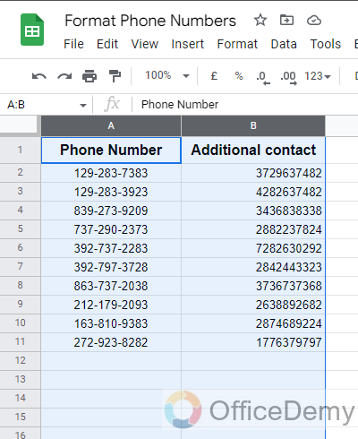
I have the formatting created for the phone number list.
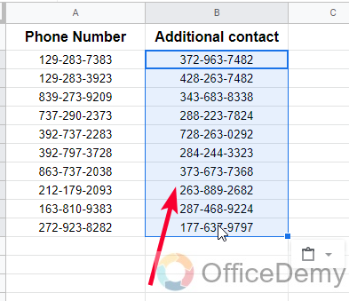
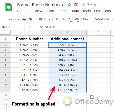
Step 2
Now I have another list that has additional contact numbers for people, here we have equal digit counts for both of the numbers so we can easily copy and paste the formatting from one list to another.
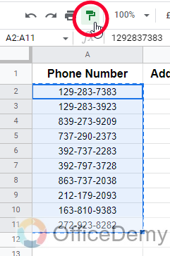
Step 3
Select the column from the column header, or select all the values in the formatted column and go to the paint format button format in the toolbar and click on it.
The format has been copied.
Step 4
Come to the destination column and select the range to which you want to apply this formatting.
As you leave your mouse you will see the formatting has been pasted to a new column and now, they both are in the same format.
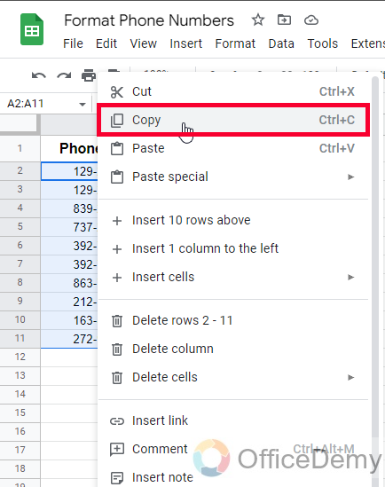
Step 5
You can also use the simple copy method, select the formatted column, and press Ctrl + c or right-click and select Copy button from the context menu.
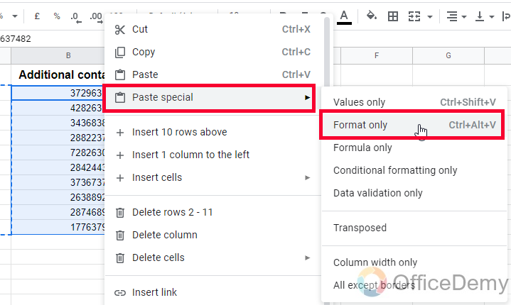
Step 6
Now go to the destination column, press Ctrl + Alt+ V, or right-click and select Paste Special > Format only.
This will also paste your format to the selected range.
Format Phone Numbers in Google Sheets – Remove Existing Formatting
Sometimes, we must change, or we may have done something wrong so now we need to remove or change the formatting applied to our phone numbers. So, for such cases, we also need to know how to remove existing formatting from phone numbers. Depending on how you have received the phone number information in your spreadsheet, you may check them first and only allow with the right formatting. Let’s see how it’s done.
Instead of making something to treat all the phone numbers with equal format, it’s better to come up with no format, and then give a new suitable format to all the numbers. Here, we have a formula that will help us do it.
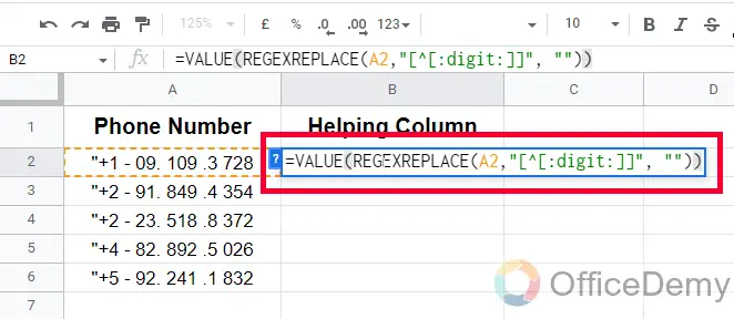
The following steps explain how to remove formatting using the formula =VALUE(REGEXREPLACE(*selected cell*,”[^[:digit:]]”, “”)) which removes all non-digit values from a cell.
Step 1
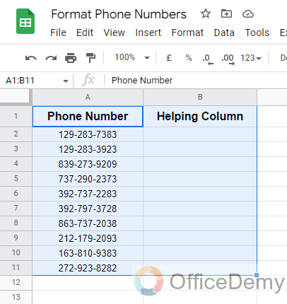
First, we need to have a column in which we have pre-formatted phone numbers and for easiness, we will add a helping column on the right side of the existing column.
Step 2
Now we need to write the above formula in the helping column and pass the cell reference for our first column has a pre-formatted phone number written.
Step 3
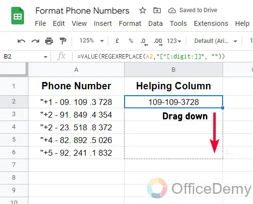
Since we have used relative cell references, we can drag this formula down to fill the column for the rest of the values.
Step 4
To get rid of the formula, you can copy all values and paste them on the same range as Values, after completing all the formula work.
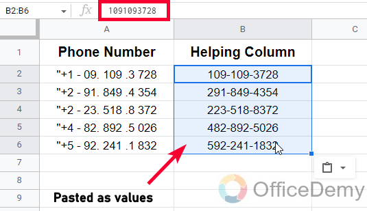
This way you will get an unformatted list of your phone numbers, and now you can give them an identical format as per your requirements.
So this is how to format phone numbers in Google Sheets. I hope you liked the above tutorial.
Frequently Asked Questions
Can the Methods Used to Remove Spaces in Google Sheets Also be Used to Format Phone Numbers?
Yes, the methods used for clearing spaces in google sheets can also be used to format phone numbers. By utilizing functions like TRIM, SUBSTITUTE, and REGEXREPLACE, you can remove any unnecessary spaces and apply a desired format to phone numbers within the spreadsheet. These techniques aid in maintaining consistency and readability in your data analysis or any other task that involves phone number formatting.
How to Format phone numbers in Google Sheets?
To format a phone number in Google Sheets, first, select the cell or cells containing the phone numbers. Then, right-click and select “Format Cells” from the drop-down menu. In the Format Cells window, select “Number” from the category list, and then select “More Formats” from the bottom of the window. From there, you can select a predefined phone number format or create a custom format.
Can I format multiple phone numbers at once in Google Sheets?
Yes, you can format multiple phone numbers at once in Google Sheets. To do this, select all of the cells containing the phone numbers you want to format. Then, right-click and select “Format Cells” as described in the first FAQ. The formatting will be applied to all of the selected cells at once.
How to format phone numbers with different international codes in Google Sheets?
To format phone numbers with different international codes in Google Sheets, you can use a custom format. In the Format Cells window, select “Custom” from the category list and enter the desired format, including the appropriate international code placeholder. For example, to format phone numbers with the +44 international code, you could use the format “+44 ###-####-####“.
How do I remove formatting from phone numbers in Google Sheets?
It’s pretty easy, simply select the cell or cells containing the formatted phone numbers. Then, right-click and select “Clear formatting” from the drop-down menu. This will remove all formatting, including any phone number formatting, from the selected cells.
How to format phone numbers in Google Sheets with a specific format?
To format phone numbers with a specific format in Google Sheets, select the cells containing the phone numbers. Then, right-click and select “Format Cells” from the drop-down menu. In the Format Cells window, select “Number” from the category list, and then select “More Formats” from the bottom of the window. From there, you can select a predefined phone number format or create a custom format that matches the desired format.
Conclusion
Today we learned, how to format phone numbers in Google Sheets. I tried to cover all the things inside this tutorial and I have shown you how you can create your custom phone number formats within Google Sheets, how to copy the formatting of the custom phone numbers format, and how to remove or change this formatting from phone numbers. With that said, I will see you soon with another useful guide. Thank you so much for reading our tutorial. Keep learning with Office Demy.


