
To Highlight Rows and Columns in Google Sheets
- To highlight empty cells, select the data range.
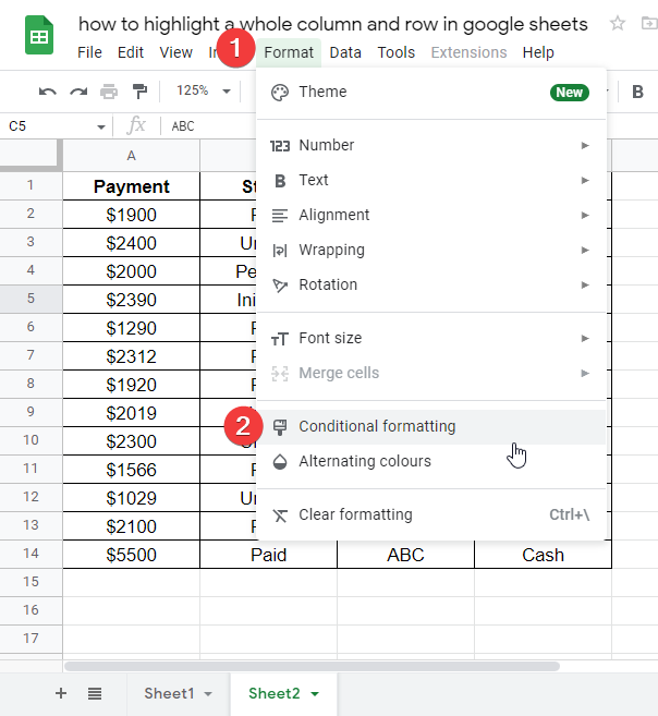
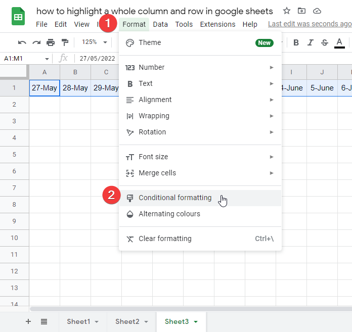
- Go to “Format” > “Conditional formatting“.
- Set a condition (e.g., if a cell is empty).
- Choose a formatting style, and your data will be highlighted accordingly.
OR
- If you want to highlight entire columns, select the entire column by double-clicking the column header.
- Apply conditional formatting as before, but this time it will affect the entire column based on the condition you set.
OR
- To highlight entire rows, select the data range.
- Navigate to “Format” > “Conditional Formatting“.
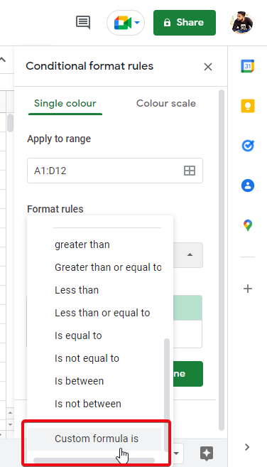
- Choose “Custom Formula is” in format rules.
- Create a formula based on the condition you want (e.g., $D2 < 20 for rows where the value in column D is less than 20) > Define a formatting style.
Hi, in this article, we will learn something like designing, so we are going to learn how to highlight a whole row and column in google sheets.
We will see examples and use cases with screenshots. We will also use conditional formatting to learn and implement how to highlight a whole row and column in google sheets. This is very important when we have a lot of data and we want to highlight entire rows or columns based on some conditions, conditions can be anything, a date, a value, a text, a number, a function, or anything we will see multiple use cases in detail. For your overview it’s done using conditional formatting, we define our condition and the formatting is applied only when the condition becomes true.
Why do we need to learn highlighting row and column in google sheets?
We regularly deal with a lot of data that may have a lot of redundancies that we don’t know, and also, we can’t perform it manually because managing and manipulating large data sets manually can lead to data loss, and you will never like it. So, we have many functions and methods to perform on the data to get easy modeling and data analysis. From this article, we will learn to identify specific data by conditional formatting that cannot be found manually. So, let’s understand how the process works.
How to Highlight a Whole Row and Column in Google Sheets
Step by Step procedure to learn how to highlight a whole row and column in google sheets is not that difficult, the important thing is that you should have some basic knowledge of formulas and functions used in conditional formatting, but if you don’t know, don’t worry I will cover it from the very basic.
We are working on a very basic example to understand how to highlight a whole row and column in google sheets. It will help you understand how it works, and also introduce you to conditional formatting if you are a newbie.
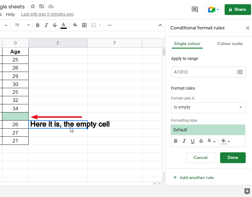
How to Highlight Empty Cells in Google Sheets
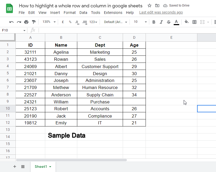
So, in this example, we will detect the empty cells by applying conditional formatting and we will format column and row to detect the exact cell address
Step 1: Fill some random data into your google sheet file
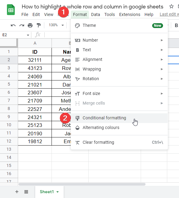
Step 2: Go to Format > Conditional formatting
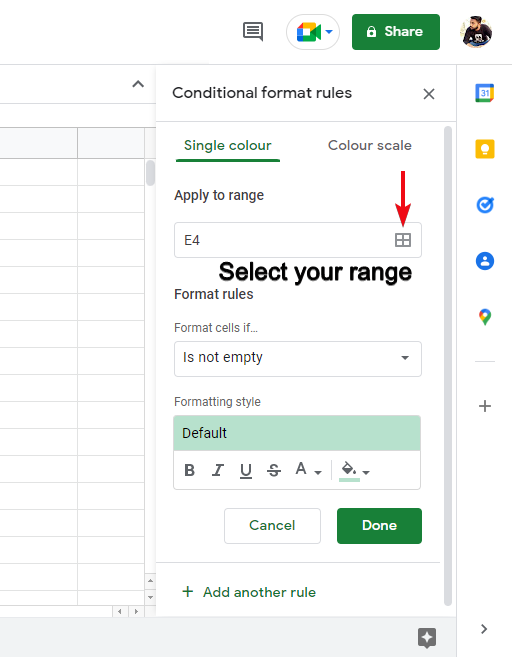
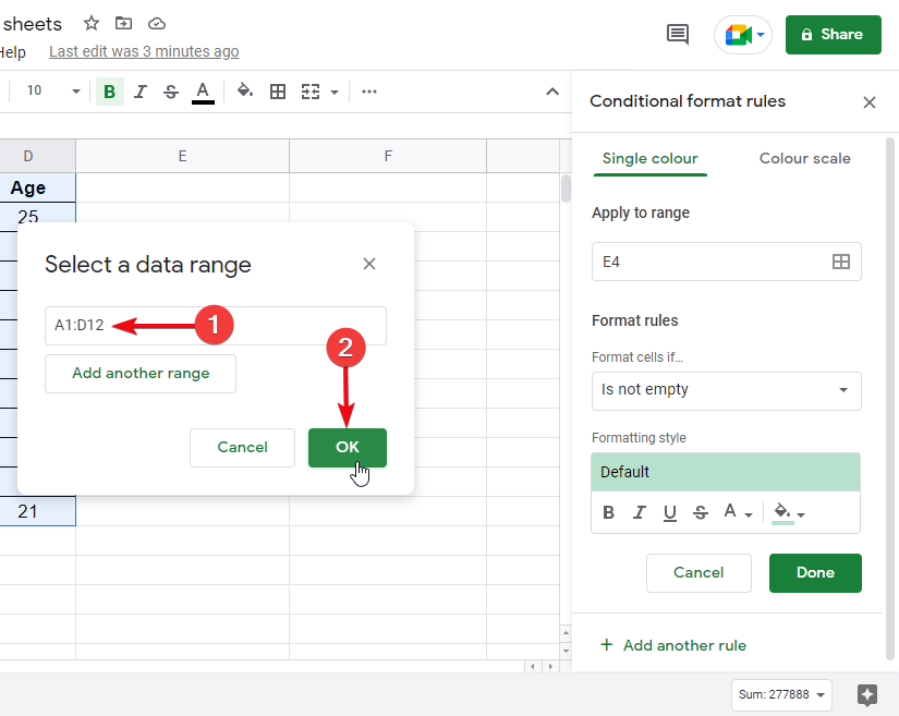
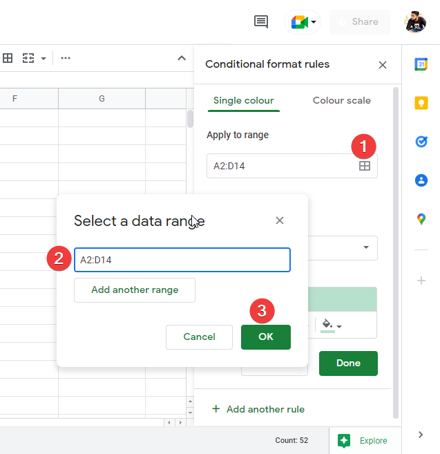
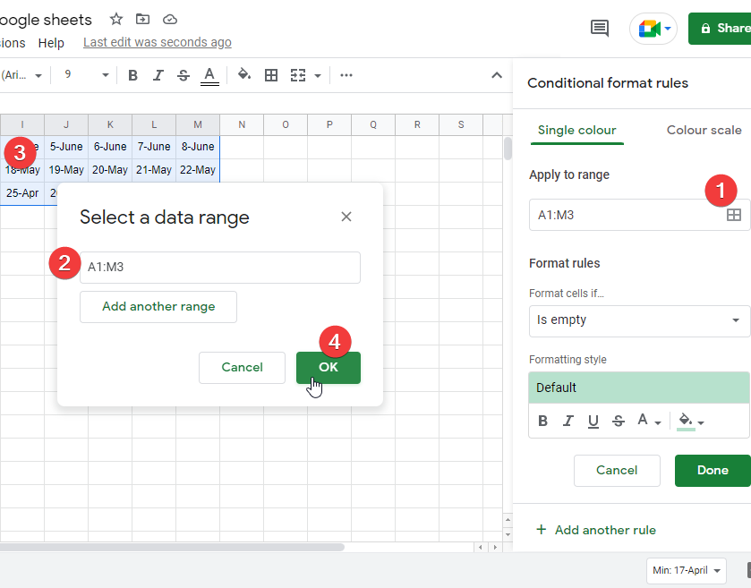
Step 3: Click on the icon in the “Apply to range” section to select the date range
Step 4: Provide range
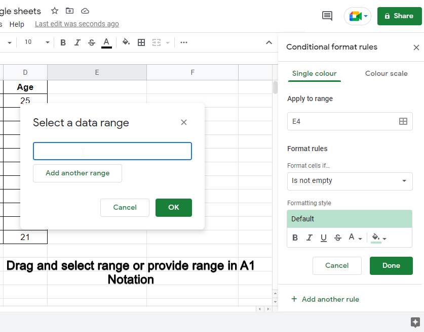
Step 5: Click Ok after providing the range
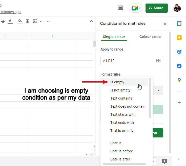
Step 6:
In format rules > select a condition
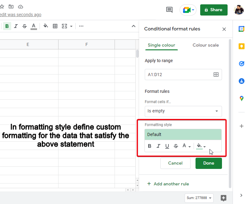
Step 7: Set Formatting style
Step 8: Click done and see your data should be highlighted.
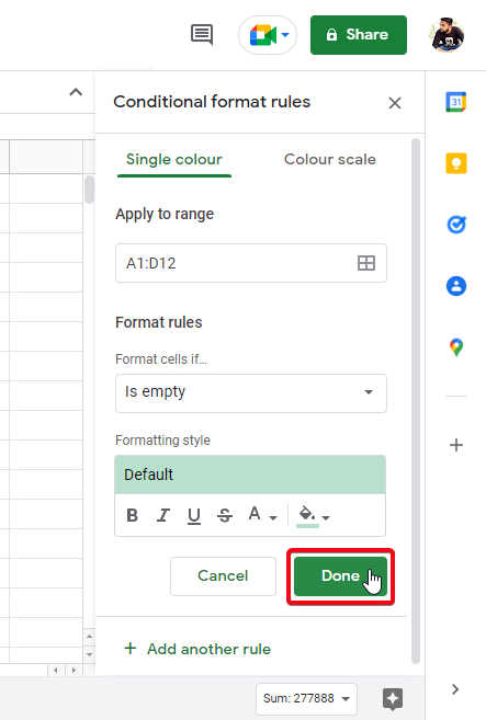
This is how easily we can detect empty cells using conditional formatting in google sheets and highlight them.
How to Highlight a Whole Column in Google Sheets
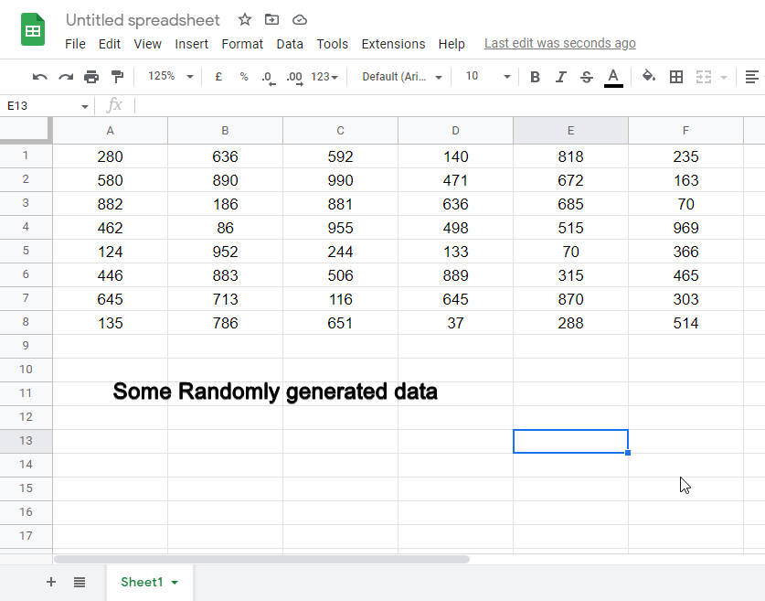
In this section, we will perform the alternative work, instead of rows, we will highlight entire columns based on a certain condition. In this example, I have generated random numbers between 1-1000 using Floor.Math and Random Formula combination, these number changes on edit, so for practicing this random numbers are too good and highly suggested.
The formula I used for generating random numbers
=FLOOR.MATH(RAND()*1000)
Step 1: Generate some random Numeric Data
Step 2: Go to Format > Conditional Formatting
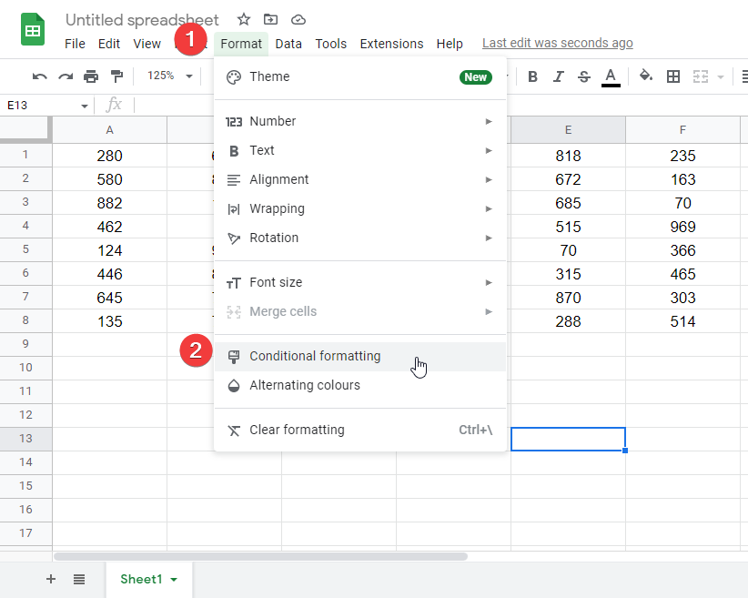
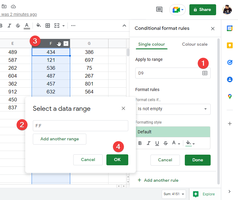
Step 3: Select the range, double click on a column header to select the whole column, then click OK
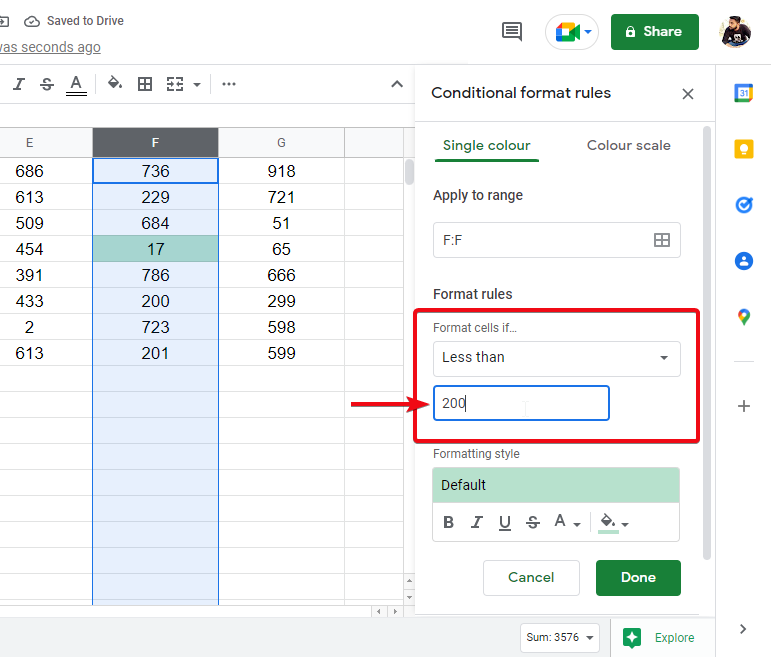
Step 4: Click on Format Rules > Less Than
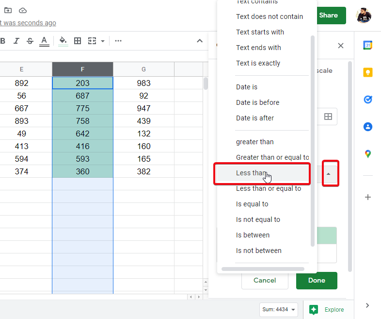
Step 5: Provide any numeric value between 2-999
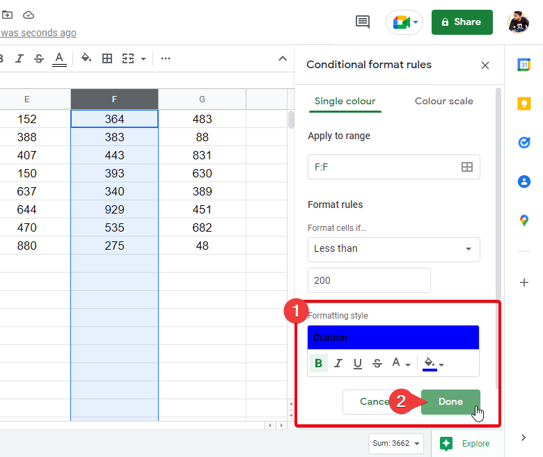
Step 6: Choose Formatting Style and click done.
Step 7: Since these numbers are randomly generated, now see the behavior of formatting on every change
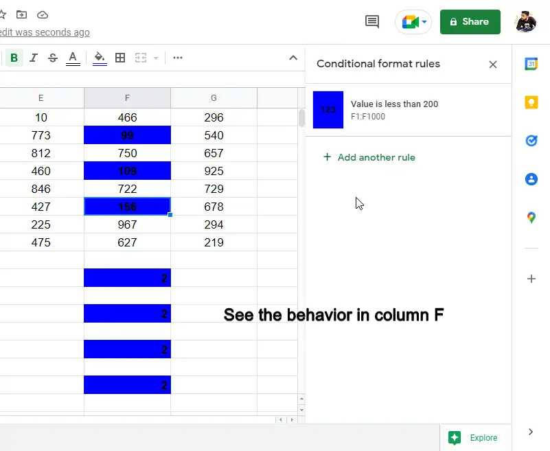
This is how you can easily use the above steps to highlight a whole column in google sheets
.
How to Highlight a Whole Row in Google Sheets
Sometimes, we don’t want to highlight a single cell or some cells we need to highlight a whole row in google sheets for some reason. So, in this section, we will see how to highlight a whole row in google sheets with the help of the same conditional formatting methods.
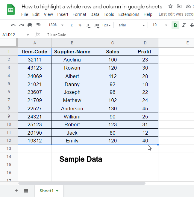
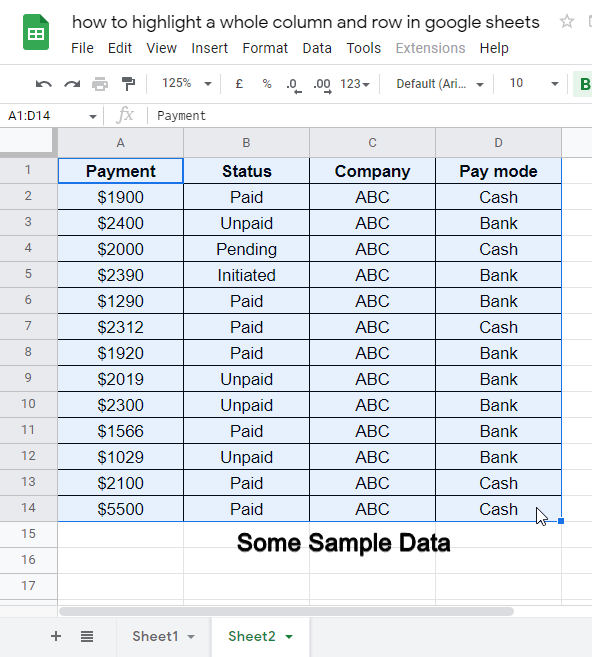
In this example, we will see data on sales, and we will apply the conditional formatting rule for the profit column in which we will detect if any value in the profit column is less than 20, if so, the whole row should be highlighted.
Step 1: Sample data
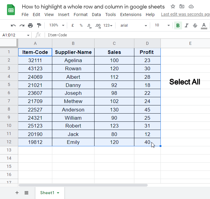
Step 2: Select all
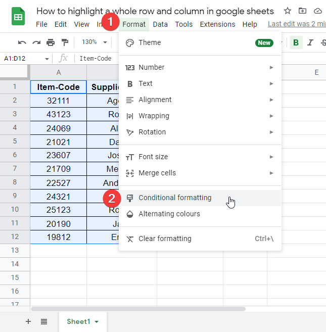
Step 3: Go to Format > Conditional Formatting
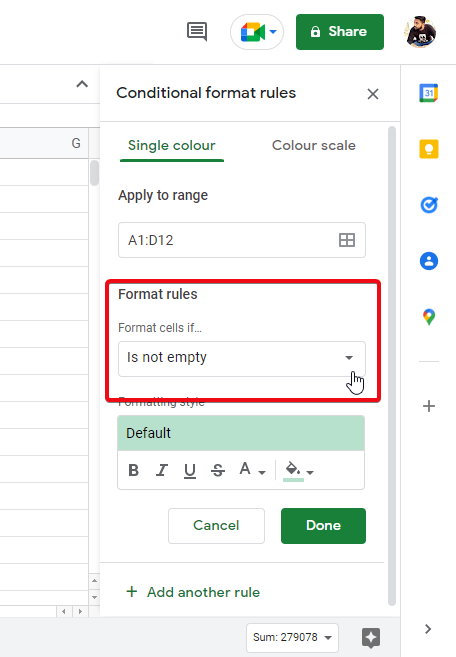
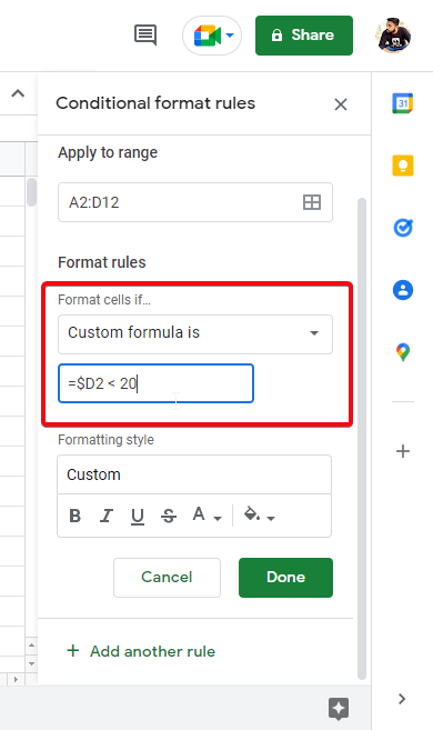
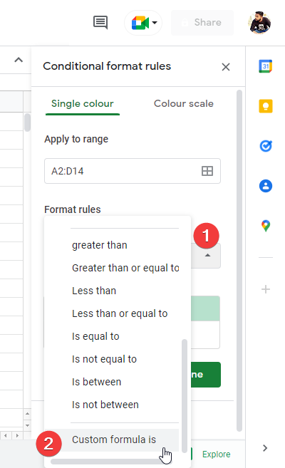
Step 4: In Format Rules > Select “Custom Formula is”
Step 5: Manipulate the formula according to your need, I used the below in the example
=$D2 < 20
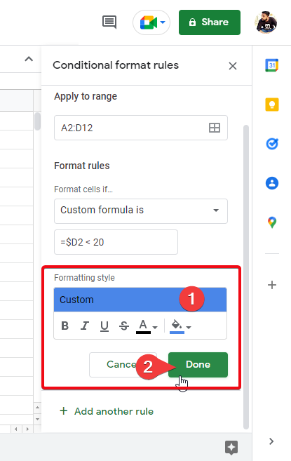
Step 6: Choose Formatting Style and click done.
This is how you can easily use the above steps to highlight a whole row in google sheets
How to Highlight a Whole Row in Google Sheets based on a String Value
In previous sections we simply saw how to highlight a whole column and row in google sheets, now very specifically we will see in this section, how to highlight a whole row in google sheets based on a string value, we will match a string and based on the true or false condition we will apply conditional formatting for one possibility.
Step 1: Get some sample data
Step 2: Go to Format > Conditional Formatting
Step 3: Select the entire data (excluding headers), and click Ok
Step 4: In format rules: select “custom formula is”
Step 5: Enter the formula
=$B2 = “Paid”
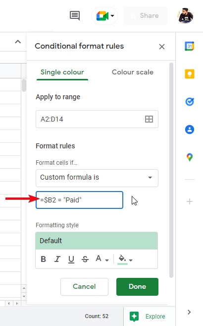
Step 6: Set Formatting Style and click done.
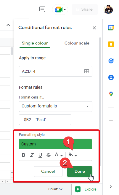
Step 7 (Optional):
Similarly, you can do the same for other string values in column B, with red color for unpaid and yellow color for pending. Try it to improve your practical skills. Good Luck!
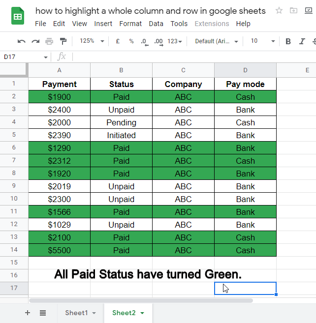
So, this is how simply you can highlight a whole row in google sheets based on a string value.
How to Highlight a Row or Column based on Dates (today, tomorrow, last week, etc.)
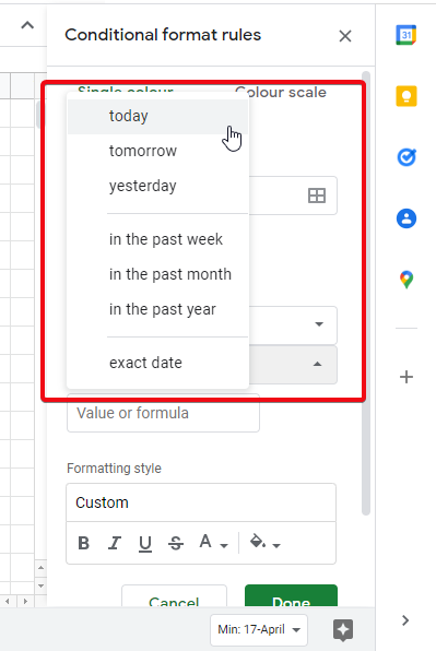
So, in this section we will see how to use conditional formatting based on dates, date can be defined using the pre-defined date methods in google sheets, we will see all the available date options and learn how to highlight a row or column based on dates (today, tomorrow, last week, etc.). So, let’s see how it works.
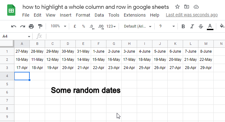
Step 1: Write some random dates
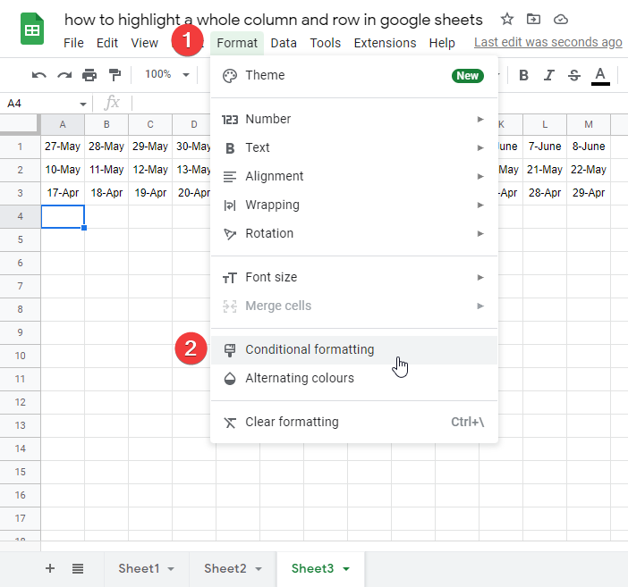
Step 2: Go to Format > Conditional Formatting
Step 3: Select the entire range of dates
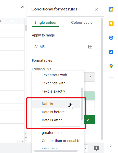
Step 4: In Format Rules > select Date is > any date option
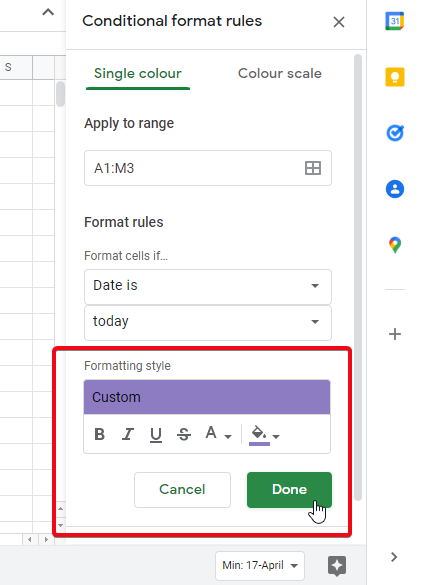
Step 5: Set Formatting style, and click Done
This is how you can simply work with dates and format them in conditional formatting.
How to Highlight Dates within a Range
So, as you saw in the previous section that how we can work on dates and format them with conditional formatting rules, but we used pre-defined methods that provide limited functionality. So, here is another section that will go a little deeper into the dates, and we will teach you how to format some specific dates over the duration of time. So, let’s learn how to highlight dates within a range.
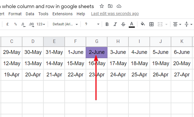
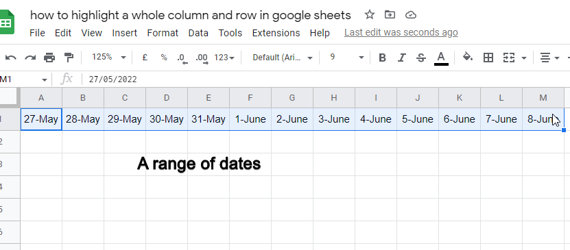
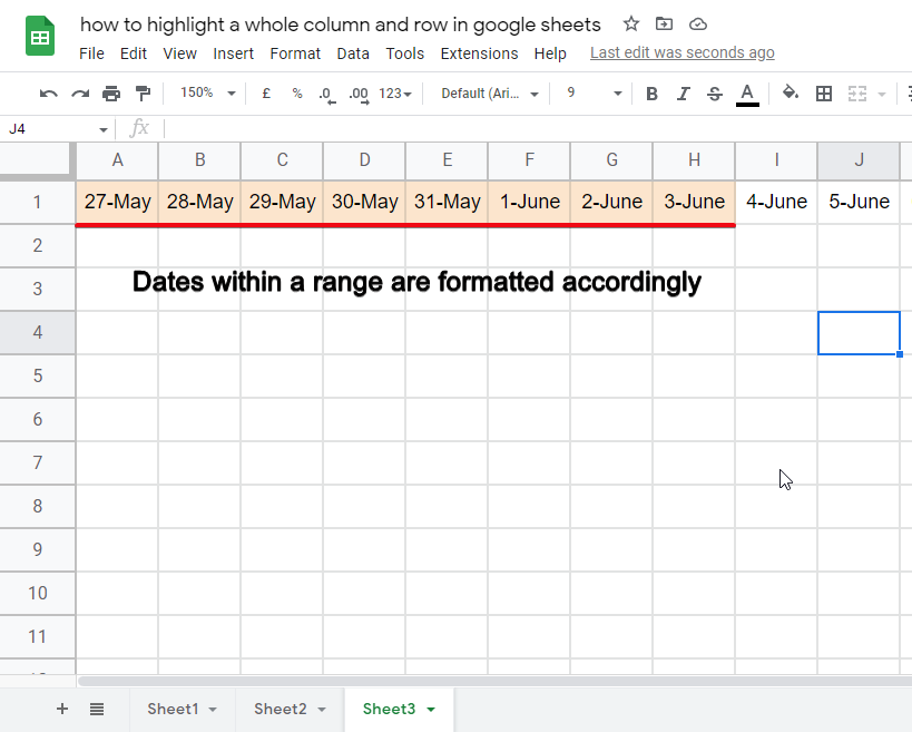
So, in this example, we have some dates ranging from 27-May to 8-June. We want to highlight some dates under a particular range (e.g.,) from 29-May to 4-June, and anything like that so will use a custom formula for this let’s see the steps to implement this formula.
Step 1: Write some dates within a range
Step 2: Go to Format > Conditional Formatting
Step 3: Select entire range
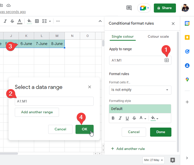
Step 4: In Format rules > Custom Formula is
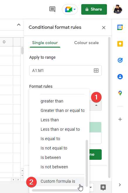
Step 5: Write the formula
=and(A$1>=date(2022,5,27),A$1<=date(2022,6,3))
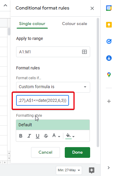
and: and is used for validating all conditions, it is true only when all conditions are true, we need to evaluate that the formatted dates should be after 27-May and before 6-June, that’s why we used =and
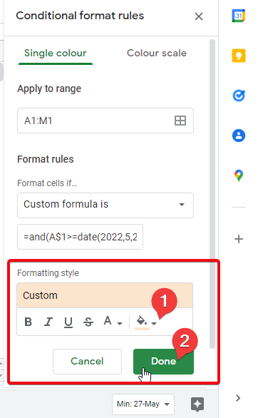
Step 6: Set Formatting Style and click Ok, you’re done.
This is how easily you can define your formula in the custom formula section, and you can do almost anything with the custom formula and get the conditional formatting.
Some Important Notes
- You can use the pre-defined conditions in conditional formatting to format your data with basic conditions.
- The “custom formula is” section provides you the power to write your custom formula/condition to format your content according to that condition and trust me you can do anything using a custom formula.
- If you have a dataset, try to write your formula on the sheet and test it to see how it works if it works fine then copy it and paste it into the custom formula is a section, the reason is that you can have suggestions when writing formula on your sheet.
- You have seen we sometimes use the dollar $ sign with range, $A2, A$2, and $A$2:$B$4, this might be irritating, so the solution for this is the F4 key on your keyboard, just write your range in normal notation and press F4, it will automatically allot dollars where needed.
Conclusion
So that’s it from today’s article. I hope you guys love it, and in this article, we tried to cover all the fundamental and common use cases of conditional formatting for highlighting an entire column and row, we saw how can we highlight specific cells, and also we saw how to highlight the entire row when an unwanted value detected in that row, similarly for columns. We worked with dates in the last two sections, and we also saw a handy function of Math (Floor.Math) with rand function to get the random numbers, you can multiply this entire expression with a number that would be the maximum limit of the range you will be getting a random number in between.
If you like the article and have learned new things then kindly share it with your buddies and do subscribe to the Office Demy blog for more upcoming articles to boost your skills in google sheets and google docs as well. Thank you!


