
To Lock Cells in Google Sheets
Lock Specific Cells:
- Select the cells you want to lock.
- Right-click, and choose “Protect range“.
- Set permissions to “Only you” to prevent others from editing.
Note: Useful when protecting specific data from unintentional changes.
Lock Cells for Specific Users
Select cells.
Right-click, and choose “Protect range“.
Set permissions to “Custom” and add editor emails.
Note: It allows some users to edit while locking others.
Lock Selected Sheets:
- Go to “Data > Protect Sheets and Ranges“.
- Choose the sheet to lock.
- You can unlock specific cells if needed.
Note: Ideal for securing entire sheets within a shared file.
Show Warning:
- Set permissions to “Show a warning when editing this range“.
- Users see a warning when trying to edit locked cells.
- Provides a chance to reconsider changes.
- Use when you want to alert users but still allow editing.
In this article, we will learn how to lock cells in Google Sheets. Well, Google Sheets has so many exciting features that help in many ways when it comes to personalization and sharing your report to make collaboration with your team of clients. One of the best things about Google Sheets is that you can collaborate very easily. But there are also some things we need to keep in mind when sharing, we cannot share a specific part of the sheets, but if you have some kind of sensitive data, or you have some complex calculation that you don’t want to be changed accidentally by anyone then you can use Google Sheets cells locking functionality.
When sharing your Google Sheets file with other people, you can share the entire file but with some areas/cells locked, this will not allow anyone to change or remove the data. When you have different people on a sheet and each has different responsibilities, then you can lock different cells/ranges for different people. So, the entire sheet will be easily shared with everyone but they will have different locked cells which they cannot work on.
Importance of Locking Cells in Google Sheets
We can lock cells for two main purposes. The first reason to lock cells can be to stop others to make changes intentionally or intentionally to a specific cell/range. This method is used when we share the file with some people to work on specific data (not the entire file), so to save our data from being removed or changed, we lock cells and share the editor’s access with the person so that they can make changes to the file but not on the specific area of the sheets.
The second reason to lock cells can be for yourself. Yes, you can also use cell locking functionality even when you don’t share the sheet with other people. Sometimes, we are only working on the sheets but still, we have some data that is very important, and we want to make sure that we don’t make any unintentional changes to it. You may paste some data on sheets and it can replace the existing one, and this happens unintentionally very frequently. So, in these cases, we can use cell locking functionality too.
Well, there are some conditions in cell locking, we will see and implement all possible scenarios of it. So, therefore we need to learn how to lock cells in Google Sheets.
How to Lock Cells in Google Sheets?
From this section, we will see the methods to learn how to lock cells in Google Sheets. We will learn all the possible conditions that anyone may have or face when locking cells in Google Sheets. So, let’s start with some sample data on a sheets file that is restricted to the owner only, after that we will also see how it works on a shared file with different people having different accesses.
How to Lock Cells in Google Sheets – Lock Specific Cells
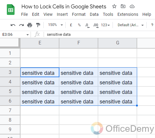
In this section, we will learn how to lock cells in Google Sheets, and we will see how to lock specific cells. In case your Google Sheets is to be shared with everyone, and some cells have sensitive data, or the data you don’t to be changed or removed by one accidentally or deliberately, this is the method for you. You can lock those cells, and whenever a user tries to change or remove it deliberately or unintentionally, they will receive a pop-up that will tell them that this range or cell is restricted by the owner and cannot be edited.
Step 1
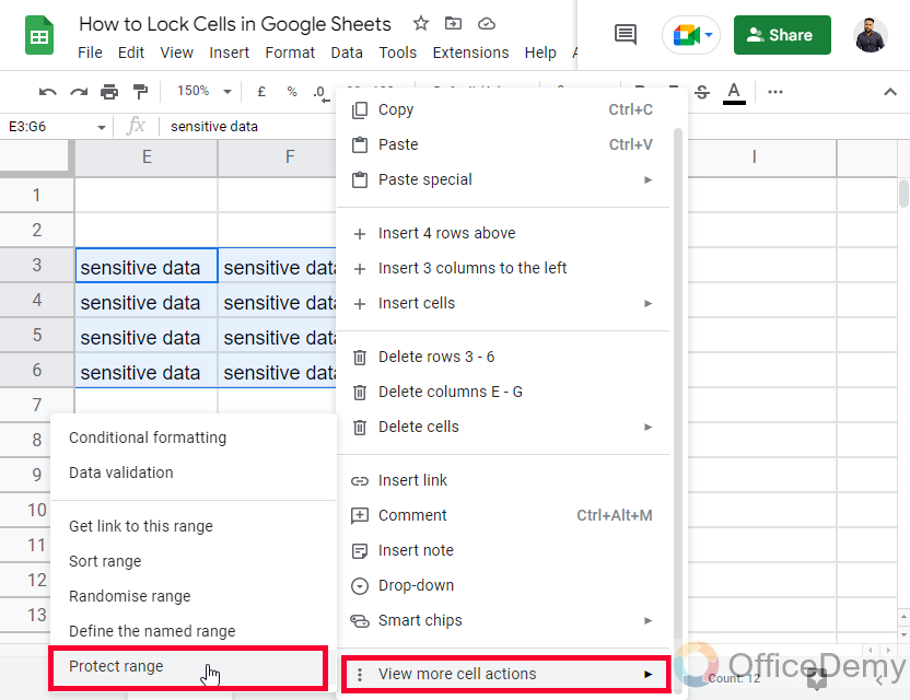
Select the cells you want to lock
Step 2
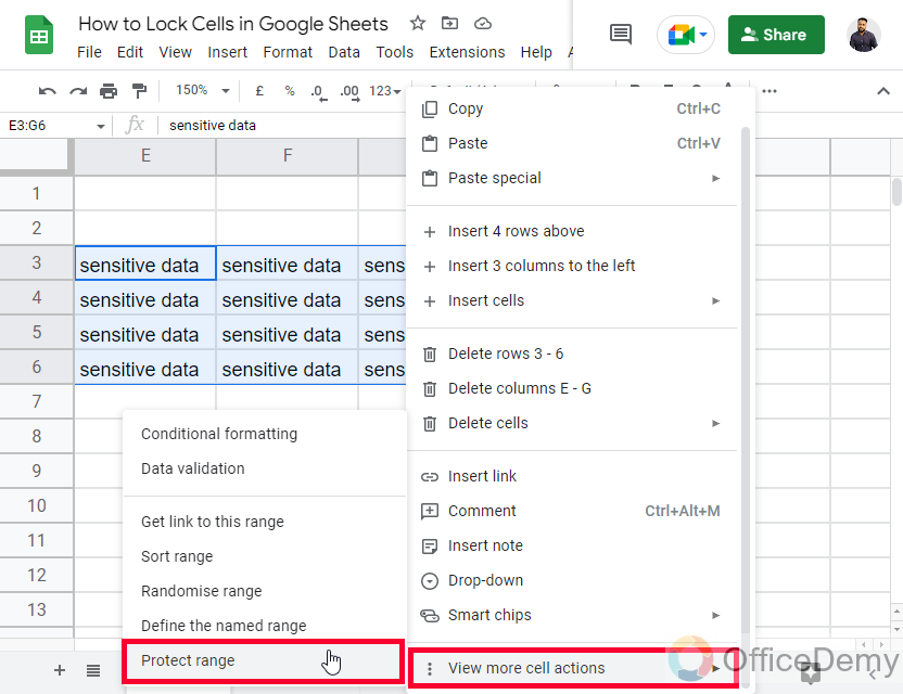
Right-click, go to “view more cell actions”, and then “Protect range”
Step 3
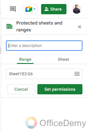
A new sidebar will open on the right side of the sheets.
Step 4
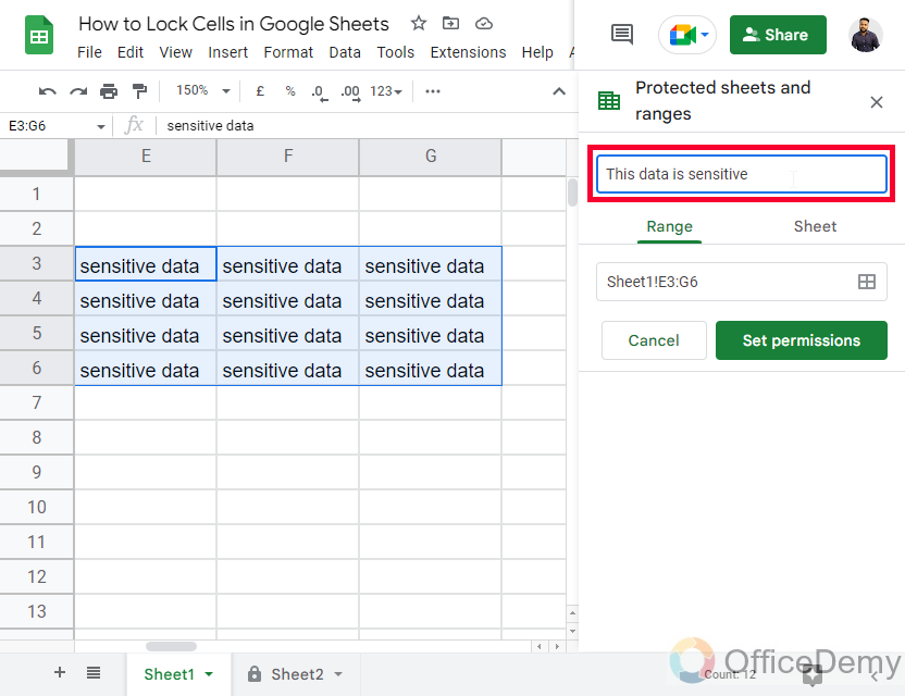
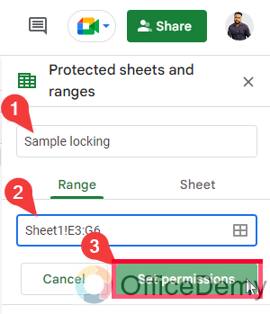
It will ask for a description, it’s an optional argument, that will help you write a reason to lock this range, which will help in the future.
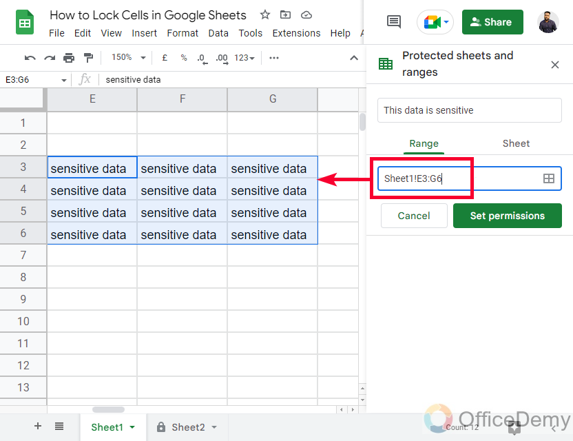
Step 5
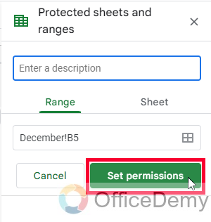
Then, below you have another input box where you need to input the cell range you want to protect
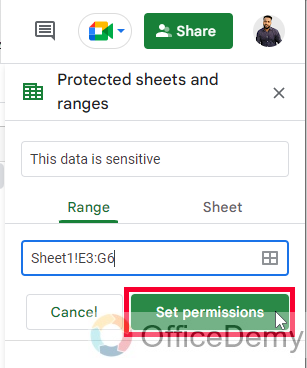
Step 6
Now you have a “Set permissions” button, click on it.
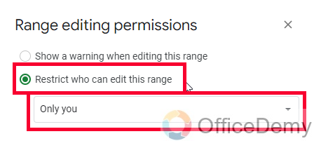
Step 7
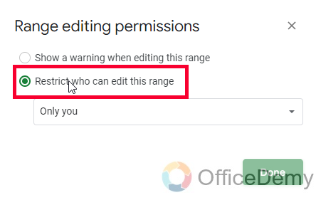
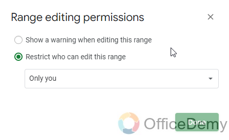
Select the second radio button “Restrict who can edit this range”, and below pick “Only you” from the dropdown.
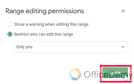
Step 8
Click Done, and now your selected range has been protected for others.
How to Lock Cells in Google Sheets – Lock Cells for Specific People
In this section, we will learn how to lock cells in Google Sheets and see how to lock cells for specific people and unlock them for others. When you have your entire team on a sheets file, and only two of them do not have anything to work with the Sheets file, but you still share with them so that can see the data, in this condition, you can lock cells only for those who have nothing to do with it. This way we can unlock cells for people who need to work on sheets, and locked for others. Let’s see how it’s done.
Step 1
Select cells or range, then right-click and go to “view more cell actions” and “Protect range”
Step 2
Give a description [Optional]
Enter the cell or range reference
Click on the “Set permissions” button
Step 3
Select the radio button “Restrict who can edit this range”
Step 4
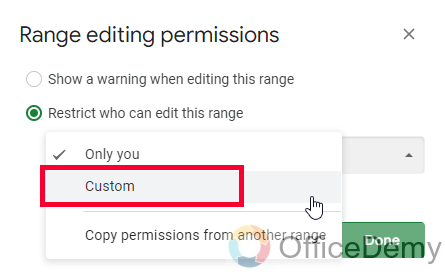
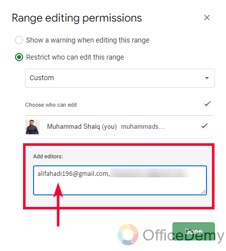
From the below dropdown, select “Custom”
Step 5
Add editors, by adding their emails, and a checkmark to them to allow them to edit the lock cells as well.
Step 6
Click on done, and then click on share, the sheets file will be shared with these people, and they can edit it, and you can also share it with others, who cannot edit it.

How to Lock Cells in Google Sheets – Lock Entire Sheets
In this section, we will learn how to lock cells in Google Sheets and specifically see how to lock entire sheets. Sometimes, we have a large workbook that has so many sheets of files in it. We want to share the workbook with our partners but there is a single sheet or few sheets that have sensitive data, and you want to protect those from being altered or deleted by anyone, so for this, we can use lock entire sheets functionality.
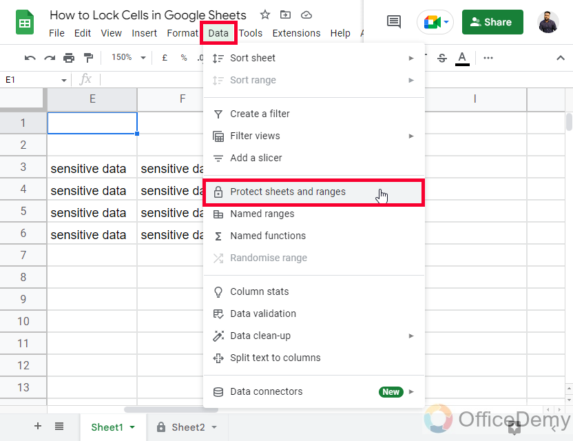
Step 1
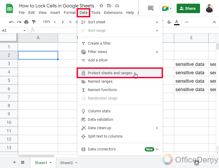
Go to Data > Protect Sheets and Ranges
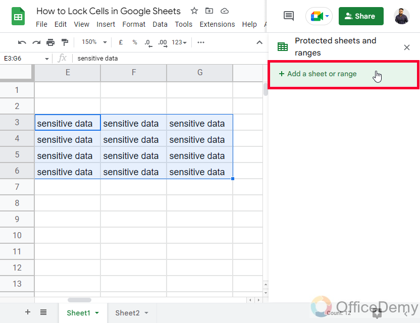
Step 2
A sidebar will open on the right-hand side.
Click on the “Add a sheet or range” button.
Step 3
You can add a description if you want [optional]
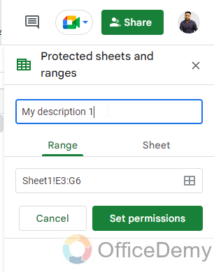
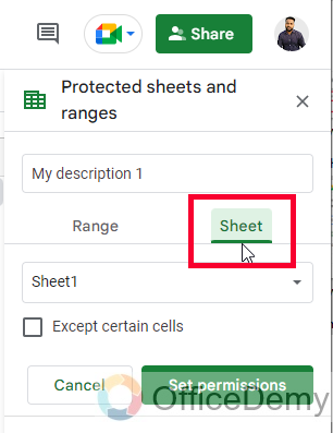
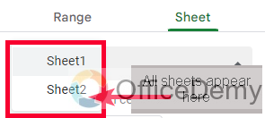
Step 4
Select the “Sheet” tab and then from the dropdown, you can select a sheet from your workbook to lock.
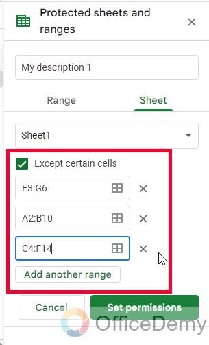
Step 5
Here, you can also use the “Except certain cells” checkbox, to protect an entire sheet but except certain cells, these will be unlocked for everyone on this file, you can select a contiguous cell range, or multiple cell ranges specifically.
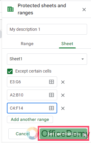
Step 6
Click on “Set permissions”
Step 7
Here, you can select the “only you” or “Custom” option to set the permissions for only you or for specific people.
This way your entire sheet will be protected.
How to Lock Cells in Google Sheets – Show Warning but Allow Editing
In this section, we will learn how to lock cells in Google Sheets, we will see how to lock cells only for a warning, and after the warning, the user can edit it. So, this method is all about letting a user know before they edit or remove the data. This method technically does not lock the cells but works as a warning message in between the “editing” and “edited” phase. This method is very helpful, when we unintentionally change some data, the sheets will change and make changes directly, but it will show a warning message, and then you can decide if you want to proceed or revert.
Step 1
After setting up your ranges to protect, go to “Set permissions”
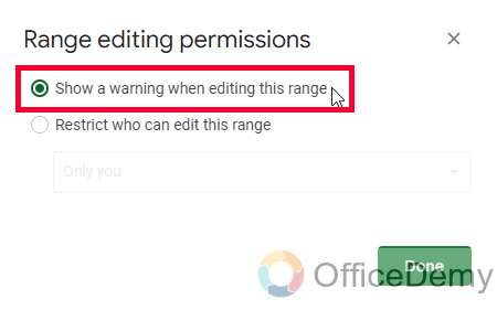
Step 2
Select the first radio button “Show a warning when editing this range”
Step 3
Click Done.
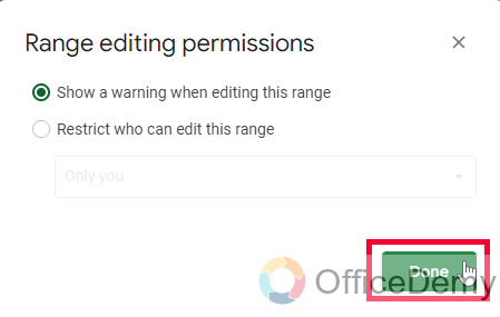
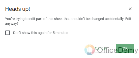
Step 4
Now, when you try to edit this range, a warning pop-up will appear, you can edit the range but this warning is only to ensure that you are editing a protected range.
How to Lock Cells in Google Sheets – Unlock Protected Cells/Sheets
We have learned four ways to lock cells in Google Sheets. Now, we must also know how to unlock protected cells and sheets. So, in this section, we will learn how to unlock protected cells or sheets in Google Sheets. Let’s go through the steps.
Step 1
Go to Data > Protected sheets and ranges
Step 2
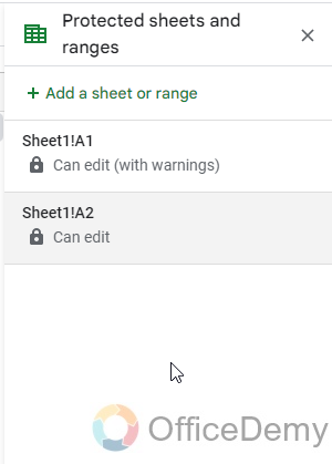
Here you have all the protected ranges and sheets, if you used descriptions when locking, you will get the description here that will help you identify the ranges, and for sheets, there are sheets names.
Step 3
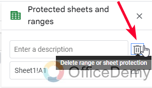
To unlock any of them, simply click on them, and then click on the trash icon in front of the description box
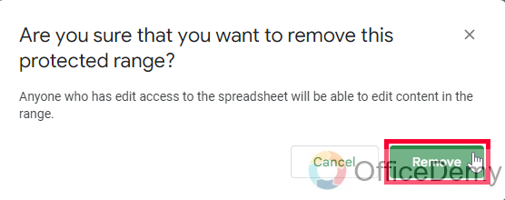
Step 4
A confirmation pop-up will appear, click on “Remove” to proceed to unlock the protected cell or range.
This is how to unlock protected cells in Google Sheets. I hope you find the above tutorial helpful.
Useful Notes
- When you are in the list of protected ranges, you will see a green border on the cell/range when you hover over its protected range
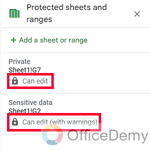
- In this list, you can also see the permissions, such as “can edit”, “can edit (with warning)” and so on. This help to identify ranges more precisely.
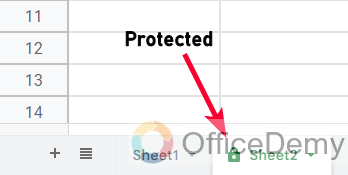
- You will also see a lock icon on the sheet which is protected.
Conclusion
This was all about how to lock cells in Google Sheets. I hope you have learned it and now you can easily lock and unlock your cells in Google Sheets. I will see you soon with another useful guide very soon. Have a nice Day! and keep learning with Office Demy.


