
To Lock Formulas in Google Sheets
- Go to the “Data” tab.
- Protect Sheets and Ranges.
- Select the cell or range containing the formula.
- Set editing permissions.
- Click “Done” to lock the formula.
OR
- In “Protect Sheets and Ranges,” click “Change permission“.
- Select “Custom” and enter the email address of the user you want to share with.
- Click “Done“.
In this article, you will learn how to lock formulas in Google Sheets. Google Sheets is a great way to collaborate with people. But sometimes it negatively affects your spreadsheet. So, if you feed complicated formulas in your spreadsheet, you would surely like to protect them from any accidental and unwanted edits by you or other users.
The interesting thing is there are different levels of protection that you can apply to any range to prevent unwanted changes. If you trust other users and want to give them access to do some important edits so you can simply use the warnings options to make them alert. Also, if you think other users might attempt to edit your formulas that you don’t agree with, you can completely prevent them from making edits.
Thus, the purpose of this write-up is to help you learn an important skill which is how to lock formulas in Google Sheets. It would be very interesting for you to learn this skill which is of great use. We have explained each step in detail which will let you understand it easily. So, carry on reading this article and follow the given instructions to learn how to lock formulas in Google Sheets.
Importance of Locking Formulas in Google Sheets
Nobody wants to waste all their hard work with some stupid blunders. When a spreadsheet is shared by more than one user, there is a greater chance of error. You will understand its importance when you invest your time to enter complex formulas. As you know only a little mistake in formulas is enough to make all values wrong. So, to minimize the chances of error and prevent your spreadsheet from unwanted edits it is important to learn how to lock formulas in Google Sheets.
It not only prevents users from making changes in formulas but also prevents them from deleting them. Note that if you try to delete the cell in which you insert the formula it will give a warning message. You are still able to delete that cell, but the formula will remain intact.
Therefore, to meet your expectations, we are here with this article that contains a complete procedure to explain how to lock formulas in Google Sheets in different ways. So, tighten your seat belts, we are now moving towards a step-by-step procedure to achieve our milestones.
How to Lock Formulas in Google Sheets
The procedure of locking the formula cells is much easy as compared to your thoughts. In this section, we will show you how to lock a formula in Google Sheets formulas. This is important to keep your formula working once you copy the cell containing it down a column or along a row. Fortunately, Google Sheets provides a couple of different levels of protection that can be applied to ranges. Read on to learn how to use these features to protect your formulas. Just follow the simple steps below,
Step 1
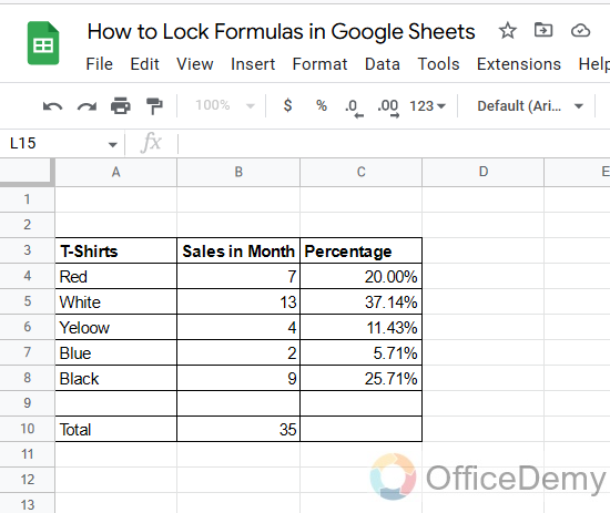
This is our sample data which consists of some formulas and calculations in the cells. Because to lock the formula in Google Sheets, we must need data set with the applied formula.
Step 2
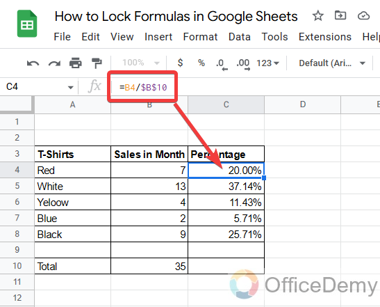
As you can see in the following picture, this cell contains a formula in it which is unlocked right now. Let’s see how we can lock this formula cell in Google Sheets.
Step 3
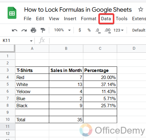
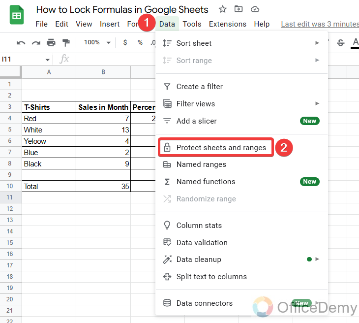
To lock the formula in Google Sheets, go to the “Data” tab from the menu bar of Google Sheets.
Step 4
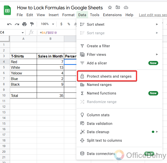
Here a drop-down menu will open where you will find the options “Protect Sheets and ranges“. Click on it.
Step 5
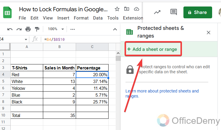
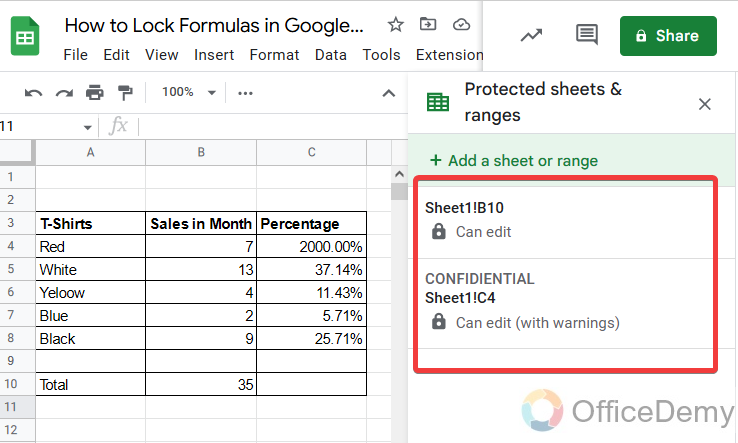
When you click on the “Protect Sheets and ranges” option, a side pane menu will appear at the right side of the window where you will find the “add a sheet or range” option. Click on it
Step 6
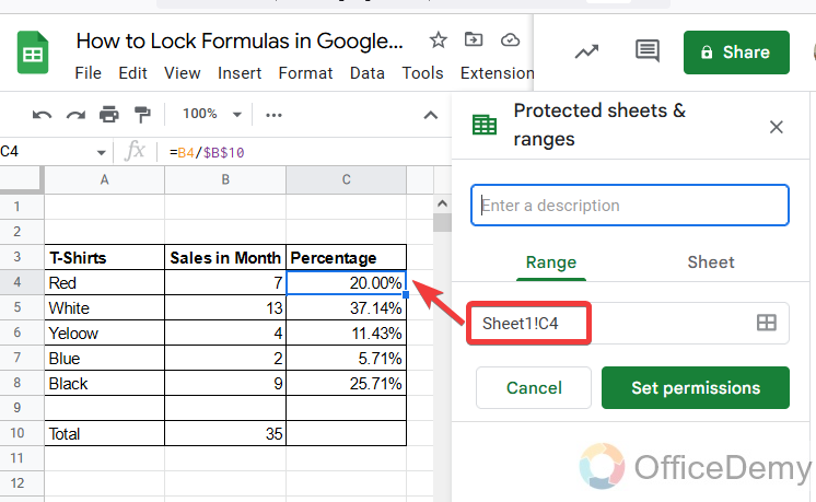
Protecting the formula cell procedure will start as click on that button, if you have selected the cell before opening the protect Sheets and ranges option then you do not need to select the range but if it is not so then select the cell where you want to lock the formula in your Google sheet spreadsheet.
Step 7
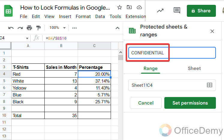
Here you can also give any message to the user that why it is protected e: g confidential
Step 8
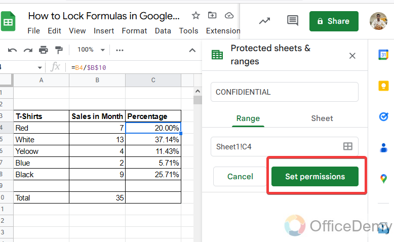
After giving the name and giving the cell address, set the permission by clicking on the “Set permission” button.
Step 9
As you click on the set permission button, a pop-up window will open like below, where you will find two options.
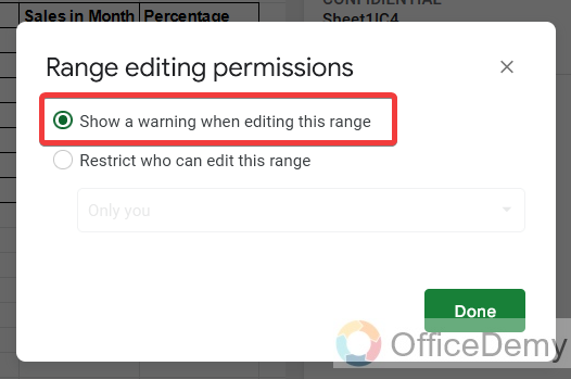
The first one is “show a warning when editing this range”. This means it will warn the person first before editing the formula after locking.
Step 10
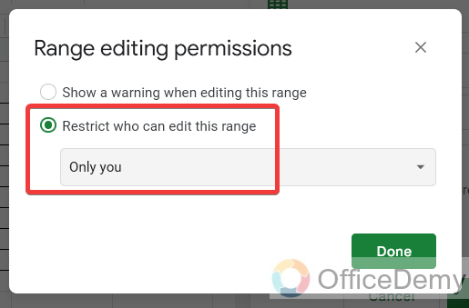
And the second one is “Restricted who can Edit this range” and the next option is “only you”. This means it will restrict the formula cell to only you. Nobody else will be able to edit it.
Step 11
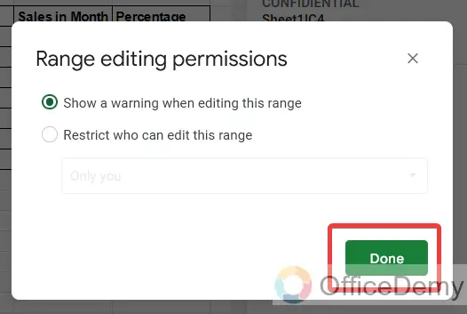
Here I am selecting the first one then we will press the “Done” button to finish it up.
Step 12
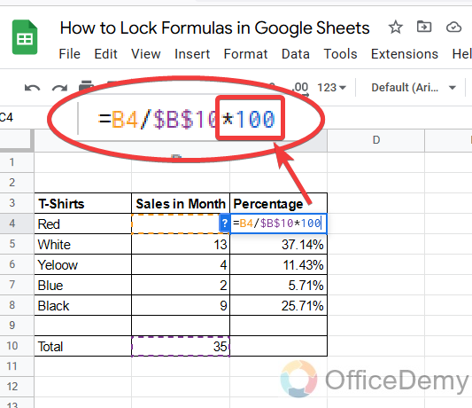
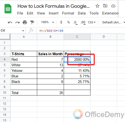
Let’s check out what happens if we edit the formula, as here I am making some editing in the lock formula cells by multiplying it hundred as you can see in the picture.
Step 13
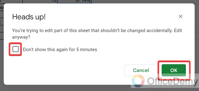
As we selected privacy, it notified first that you can read below. Although you can skip it by clicking on the “Ok” button and if you are working on the same formula for a while, you can check the option mentioned in the following picture which will not disturb you for 5 minutes.
Step 14
As you can your formula has been edited with no difficulty by clicking just the “Ok” button.
Frequently Asked Questions
Are the Methods to Lock Cells in Google Sheets the Same as Locking Formulas?
The methods to lock cells in Google Sheets differ from locking formulas. With google sheets cell locking, you can restrict specific cells from being edited while allowing formulas to be manipulated. This ensures data integrity and prevents accidental changes to essential calculations.
How can we unlock the formulas in Google Sheets?
A: There is always a key to any lock, similarly in Google Sheets if there is an option to lock the formula cells then there must be a solution to unlock it back. This is very simple to do unlocking the lock formula cells, you just need to go into the “Protect Sheets and ranges” pane menu and delete the set privacy rule for the cell range. Your cell will be automatically unlocked. Here are the steps to unlock the locked formula cells.
Step 1
To unlock the formula cell back, you will have to go back to the privacy option which you will find in the “Data” tab of the menu bar of Google Sheets “Protect Sheets and ranges” as shown below in the picture.
Step 2
A side pane menu will open where you will see your privacy rules for the formula cells. Select any of them that you want to unlock.
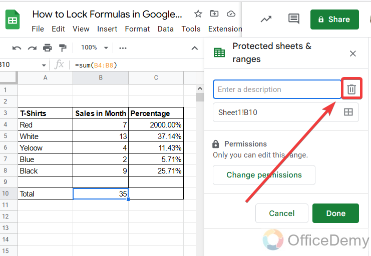
Step 3
When you click on it to edit, you will see a small Bin icon at the right side of the description option as shown in the following picture. Just click on it to remove this privacy to unlock the formula cell.
Step 4
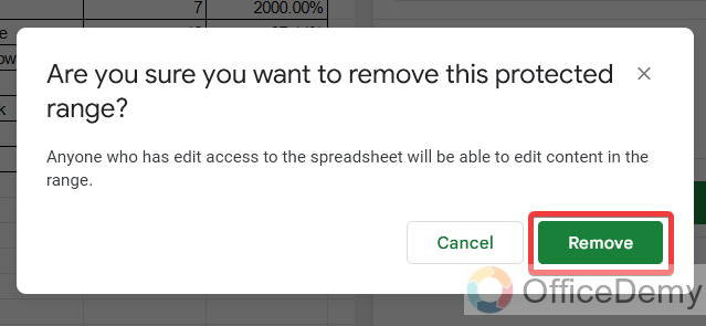
When you click on that bin button, it will promptly ask you to confirm “Remove” it. Click on the “Remove” button. Your formula cell will be unlocked.
How can we share the lock formulas with other users?
A: Google sheet is a collaborating program on which more than one or two people can work at the same time. This is why people prefer Google Sheets while working with spreadsheets. But working with a team setting up privacy can stick your partner while editing. So, if you have locked the formula cell and you want to share your privacy with your teammates then there is a way you can share with them by following the below steps.
Step 1
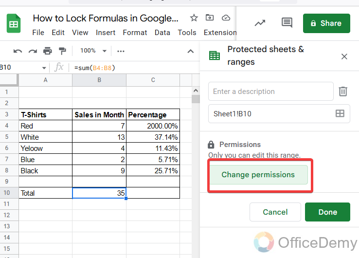
Let’s suppose you are locking the formula cell when you click on the “Change permission” button.
Step 2
It will restrict you only to editing the lock formula cells, as we discussed above.
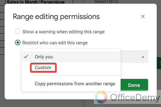
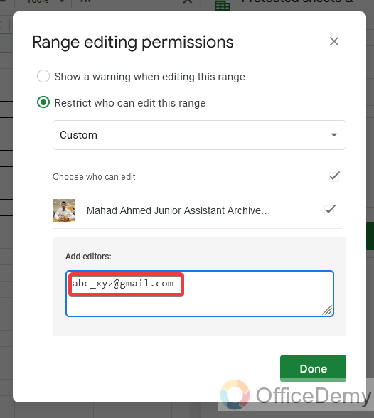
But if you want to share permission with someone to edit it, then select the “Custom” option from the following.
Step 3
You will see a dialogue box to ad editors in the prompt window, write the email address of the user with whom you want to share it to edit.
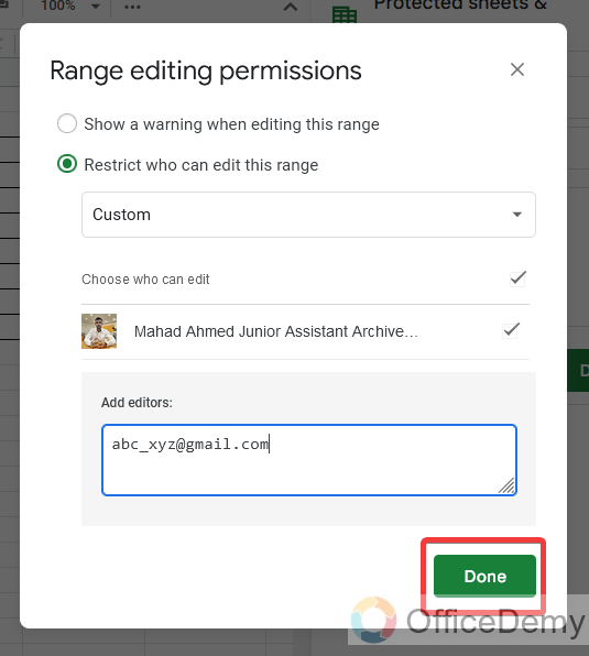
Step 4
Then click on the “Done” button, and your lock formula cell will share with the given person.
Can you lock the formula in multiple cells at once?
A: Yes! Why not if you are working with the large size of the data set which consists of many important formula cells that you want to make private or lock the formula cells? You can lock them simultaneously by just adding them in the “Protect Sheets and ranges” pane by selecting the range one by one.
Can we also lock the entire sheet in Google Sheets?
A: If you want to lock the entire sheet and want to allow viewing permission only to other users, the simplest approach is to lock the entire sheet which you can also lock with the same option. Just select the sheet instead of ranges or cells.
Conclusion
Today we learned how to lock formulas in Google Sheets. When working with a coworker in a Google Sheets spreadsheet and if you have ever written a custom formula with the time taken and want to be meticulous and willing to not overwrite it. Then the above article on how to lock formulas in Google Sheets is made for you. This will prevent you from leaving your formulas unsafe and fearing losing them, this tutorial helps you keep your formulas safe in hand and only be deleted or modified by authorized users.
You should enjoy the features of this article on how to lock formulas in Google Sheets. I will see you soon with another useful guide. Take care and goodbye.


