
To Name a Column in Google Sheets
- Select the sample data in your Google Sheet.
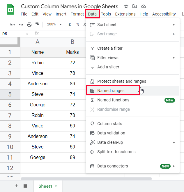
- Navigate to the “Data” > “Named Ranges“.
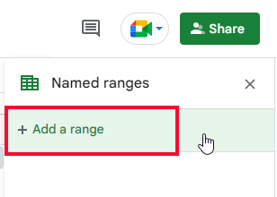
- Click on “Add a range” to define a named range.
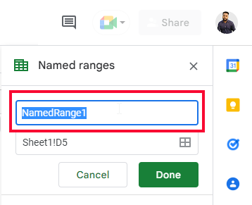
- Give a custom column name in the “Named range name” field.
- In the “Range” field, specify the range, e.g., A:A or B:B for entire columns.
- Click “Done“.
- You can now refer to your columns using the custom names you assigned.
OR
- Identify the row containing the column headers.
- Go to the “View” > “Freeze” and then “1 row“, to freeze the first row containing the headers.
- Scroll down, and you’ll notice that the headers remain visible even as you navigate through the data.
Hi, everyone in this article we will learn how to name a column and get custom column names in google sheets. We most commonly work with formulas and functions in google sheets to perform calculations and other tasks. We have a tabular layout in google sheets and we have rows and columns to work on. By default, the column names are alphabets such as A, B, C, and so on. And, similarly, row names are not names but are numbers such as 1,2,3, and so on.
When we use some cell or range inside a formula or a function so we need to pass the cell address using the cell reference which is a unique address of a cell created with the combination of column and row, s simple cell address can be A1, B4, C8 and so on. Here, we are using the column name A and then the row number 1 to refer to a cell, but what if you can use custom column names? Then you will be calling the cell like this: Sales5, Students3, Profit18:Profit29, something like this, is not it interesting? Yes, it is. So, in today’s article, we are going to learn how to get custom column names in google sheets
Why Custom Column Name is Required in Google Sheets
As you know, we mostly work with formulas and functions, so we frequently need the cell reference, the cell reference can be quickly picked up by glancing at your sheet. But, I am sure you must have experienced a situation where you are working in a below section of the site and now you can see the row number anyways because you are on that specific row, but you have to scroll up to the page to see the column name, this can be annoying sometimes.
So instead we can rename our columns and keep the names as per our needs and the context of the content we are working on. So there for the custom column names in google sheets come in the business, today we will see how to get custom column names. Although there is no direct method to do this, as always, we have two workarounds to make it possible very easily. Today we are going to see both methods.
How to Name a Column in Google Sheets
So, we have two methods for custom column names in google sheets, we will see both of these with the help of some sample data and we will apply custom column names to get easiness when working with formulas, and functions in google sheets.
Name a Column & Get Column Name in Google Sheets – using Named Ranges
As you know we have already covered the named ranges tutorial in this series of google sheets. Named ranges are an amazing addition to google sheets that allow us to have custom names for our cells, ranges, and columns. We will use the named range technique to get custom column names for our columns.
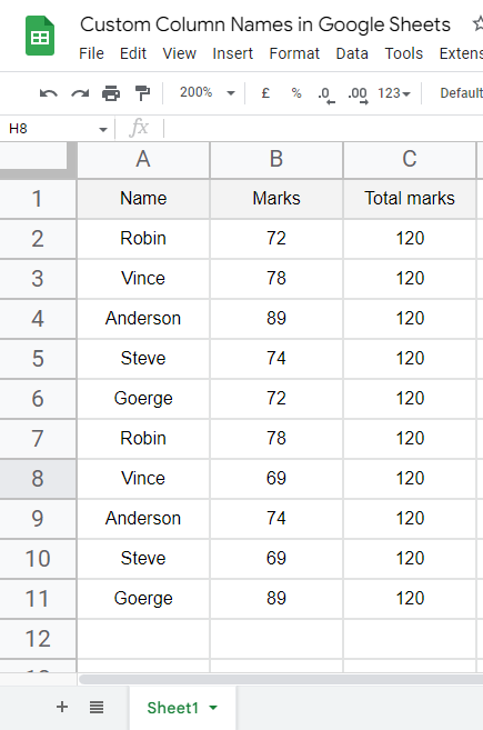
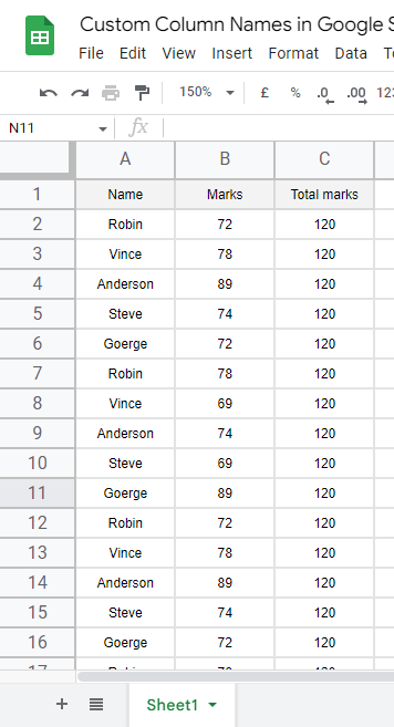
For this, I have sample data that have some student details.
Step 1
Sample data
Step 2
Go to Data > Named Ranges
Step 3
Click on add a range
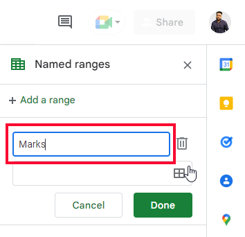
Step 4
Give a custom column name here (Named range name)
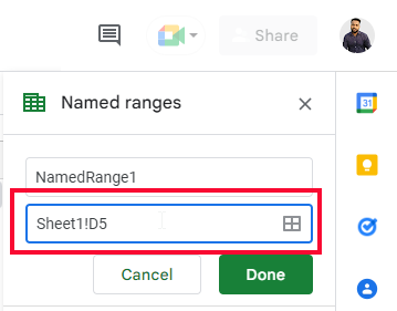
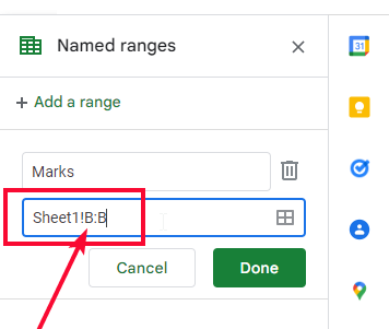
Step 5
In the below section, define the column such as A:A, B:B (this will consider the entire column A or B)
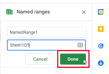
Step 6
Click on done and now you can call your specified column with the name you just assigned.
Step 7
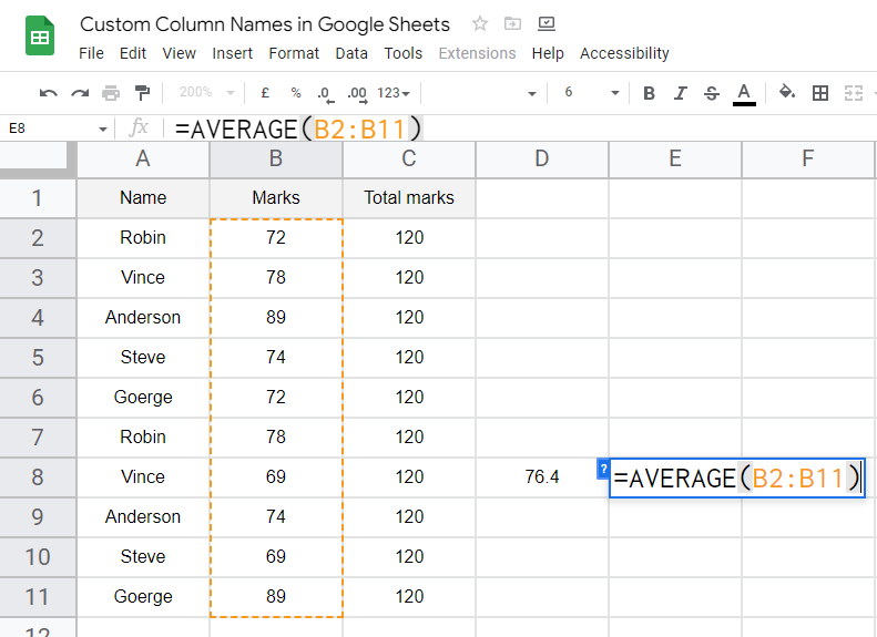
Let’s see if it works, calling a column from a custom column name
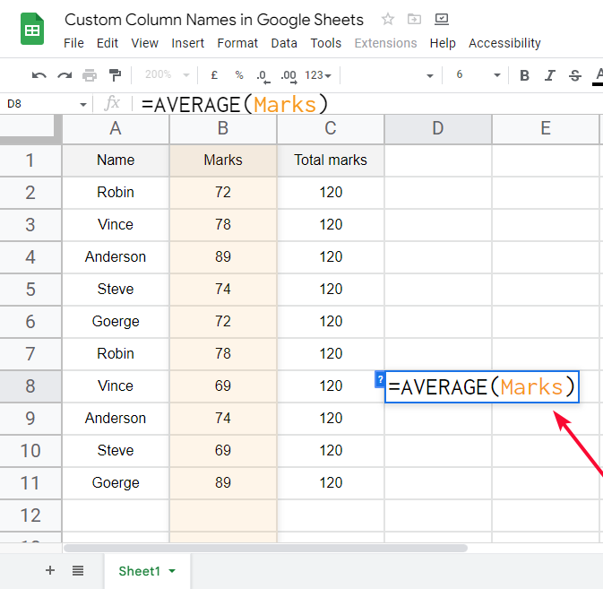
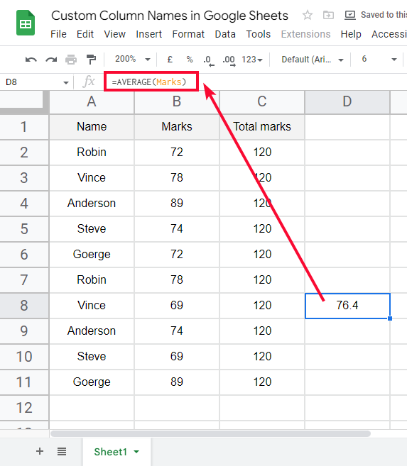
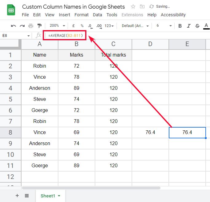
Step 8
You can see this is working perfectly.
This is the one method to get custom column names in google sheets. We can trick and can work around to have another way to do it, it’s not pretty logical but it still works and is used by many regular users of the spreadsheet
You can read a complete tutorial on Named Ranges here
Name a Column in Google Sheets – Freezing Headers
In this section, we will learn how to get custom column names in google sheets using a freezing technique. This technique is very classic and used by so many users to freeze an important row or columns for ease of working. It’s mostly done to have a sticky header on the top and does not disappear even when we scroll down, similar to the rows, if the data is horizontally aligned in your google sheets file, you can do the same thing with rows, don’t worry we will look both in detail.
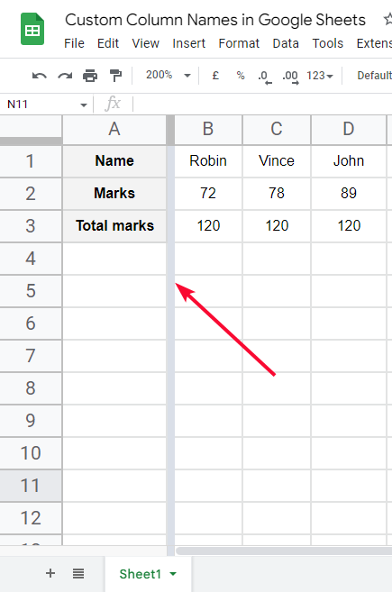
So, here for this example, I have sample data that is very long and goes on from row1 to row21. We will see how it makes it easy for us when we freeze headers and they act like the custom column names for us.
Step 1
Sample data
Step 2
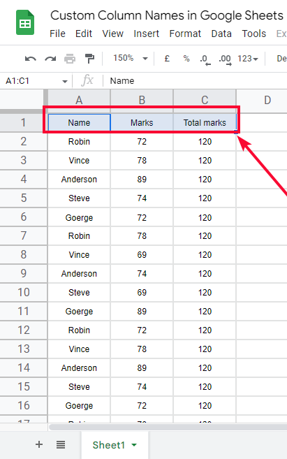
The column headers
Step 3
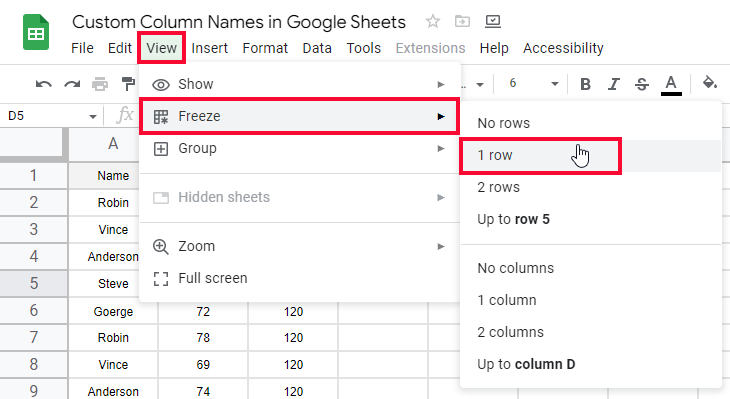
Go to View menu > Freeze > 1 row (normally 1 row because our header has one row)
Step 4
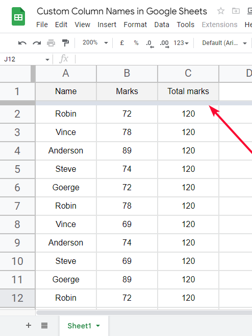
Now you can see a thin grey line below the frozen row
Step 5
Scrolling to the last row
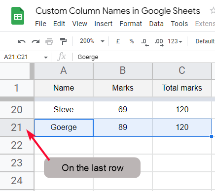
Step 6
The header is still here.
This is how we can use this header as custom column names. It was originally not the actual header of the column, but we have made it look and act alike. So, this is how we can make our header row sticky to get custom column names in google sheets.
This way, we can also change the headers accordingly, we have not used Named ranges here, so any problem even if we need to change the headers.
Now let’s see another quick scenario when you have data aligned horizontally.
Name a Column in Google Sheets – Freezing Headers for Horizontally aligned Data
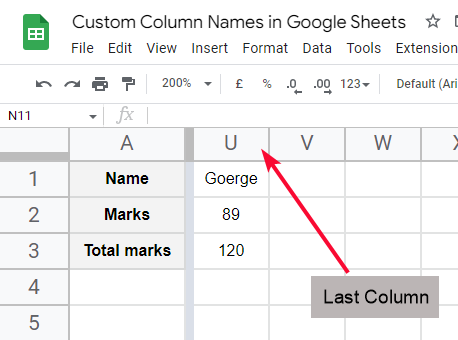
In this section, we will learn how to get custom column names in google sheets by freezing headers for horizontally aligned data, which means we have data left to right and not top to bottom, so the scrolling will also go from left to right and not top to bottom, here we can use the same technique to freeze the headers and they will not disappear even when we scroll right to the last column.
I have a similar dataset aligned horizontally
Step 1
Sample data
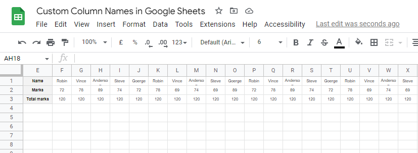
Step 2
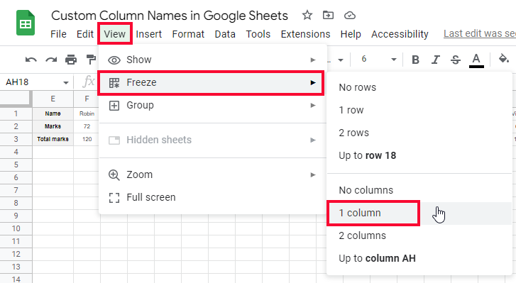
Go to View menu > Freeze > 1 column (column; because we are working on the different orientation of data)
Step 3
Again, the same thin grey line indicates that the previous area is frozen and will not disappear on scrolling
Step 4
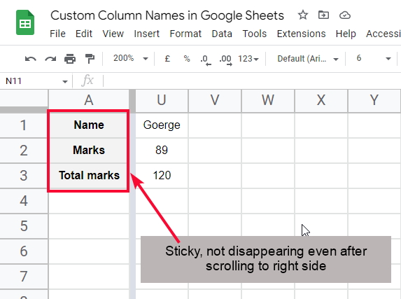
Scroll right to the right-most column
Step 5
You can see the headers are not disappeared, and they are looking like column headers and you can edit them as per your need.
These were two easy methods to get custom column names in google sheets. I hope you find this article helpful and that you have learned something new from it.
Download/Copy Google Sheets Workbook
Useful Notes
- Named ranges have some naming rules while naming your range or column, make sure that you use a valid name and avoid the restricted characters
- Named ranges must have a unique name, two named ranges cannot be of the same name, you can differentiate them as 1, and 2 labels if you have two columns with the same name
- Named ranges are different from Named functions
- You can delete Named ranges from Data > Named ranges > edit a named range and a trash icon will appear to click on it and then confirm your action to delete the named range from the sheet
- Named ranges have no limit, you can have as many of them as you need to
- Named ranges can be of ranges, cells, columns, rows, etc.
- The freezing method is good when you need to keep an eye on your data header, it’s not useful to call a range or cell by a custom name.
Frequently Asked Questions
Can the Methods Used to Split First and Last Name in Google Sheets be Applied to Naming a Column as Well?
Yes, the methods used for splitting first and last names in Google Sheets can also be applied to naming a column. By following the same process, you can easily create a column name by splitting and combining the desired words or phrases. Utilizing this method ensures efficient organization and clarity within your spreadsheet.
How do you rename column names in google sheets?
There is no direct or indirect method to rename the original column name, you cannot rename a column and change the alphabet with some custom text. There are some similar goals we can achieve using the workarounds we have learned in this article. We have addressed the problem you want to solve by renaming column names in google sheets. So, the named range method can give you custom column names for calling a column into a function or formula, and on the other end, the freezing method is used to keep an eye on your column or row headers when working on a big file with so much scrolling. The freezing method cannot call a range or column by a custom name.
I hope you find this answer helpful. You can comment below on your problem, and I will try to reach out with a simple solution.
Conclusion
Having custom column names is exciting for any google sheets user. This article was meant to give you a feel of custom column names, in this article, we learned how to get custom column names in google sheets. We discussed the benefits of having custom column names, we discussed how they help us when working with functions and formulas. The other use case is to make sticky headers using the built-in freezing function in google sheets. We can freeze the header area can be rows or columns, and then we can scroll down or right anywhere in the sheet and the headers will remain visible to us. This helps a lot when we need to use formulas and functions to pass the values. The freezing technique helps us by avoiding so much scrolling for us and showing the headers everywhere we go on the same sheet.
That’s all from custom column names in google sheets. I hope you like this tutorial and that you have got the idea behind this lesson. I will see you soon with another helping tutorial. Keep learning with Office Demy. Thank you.


