
To Remove Hyperlinks in Google Sheets
- Select a cell containing a hyperlink.
- Click on the right-most icon in the dialog box that appears (the “remove link” icon).
- The hyperlink will be removed, and the text will remain as a value.
OR
- Select all the cells with hyperlinks.
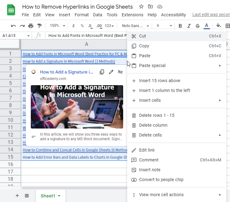
- Right-click on any selected cell.
- Go to “View more cell actions” > Choose “Remove link“.
- All the hyperlinks in the selected cells will be removed.
Hi all. In this article, we will learn how to remove hyperlinks in google sheets. Often, we have links copied from some sources, or they are some original links to navigate the site using the browser. In google sheets, we can create hyperlinks by assigning a link to a part of text or cell. But sometimes links can be annoying, the blue color, blue underline, and some special formatting make a link look different from the normal text, and for some reason, we may not want this type of formatting, or sometimes we copied some text and that was a link, and now we want to keep that text as value text, not as a link, so we need to remove those links. So, how to remove hyperlinks in google sheets is the context of this tutorial.
When we need to remove Hyperlinks in Google Sheets
Most times we copy some listicles from the internet to google sheets or google docs, and what happened, they are pasted like hyperlinks and look so annoying, there is not only the formatting that can annoy a user but also the hover effect. When you mouse over on the link a small dialog box will open below the link, and this mostly happened unintentionally we are just navigating over the sheets and when our mouse meets the link the small horizontal window of the link is opened.
So to avoid all these things, we need to learn some quick and handy methods to remove hyperlinks and keep the data as normal text or values. Therefore, we need to learn how to remove hyperlinks in google sheets. Let’s see the step-by-step procedure to learn how to remove hyperlinks in google sheets.
How to Remove Hyperlinks in Google Sheets
We have so many methods to remove hyperlinks in google sheets. Let’s start seeing those methods and have some dummy data as well to learn the methods properly.
I am copying some linked data from the internet then I will show you the behavior of links and then we will see how to remove hyperlinks very easily using various methods.
Remove Hyperlinks in Google Sheets – using Link Icon below a Link
In this section, we will learn how to remove hyperlinks in google sheets using a link icon below a link when we click or mouse over a link in google sheets. This is a very simple method, but it cannot be used to remove hyperlinks in bulk quantity, yes, this method is limited to removing only 1 hyperlink at once, you have to repeat this method for every link, so if you have bulk data this method is not suitable. But to remove a single link, can be the fastest way.
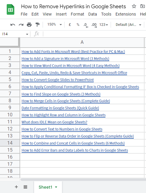
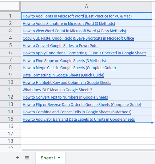
I have some simple data set below in which I have some tutorials I copied from the officedemy.com blog. This is a list I have copied for my reference, but when I paste it into google sheets, they are automatically pasted as links. Now I need to remove the links because they are annoying me
Step 1
Sample data
Step 2
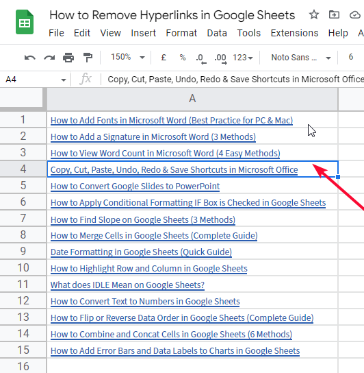
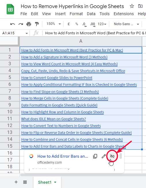
Select any cell containing a hyperlink and you will see a dialog box will appear with the link details and some icons on the top right
Step 3
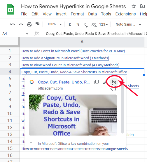
Click on the right-most icon (remove link)
Step 4
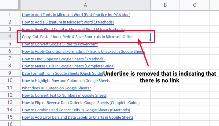
Your link is removed and the text remains as a value (you can see the underline is removed which is indicating that there is no link, and also now you cannot see any dialog box by mouseover or clicking on that cell)
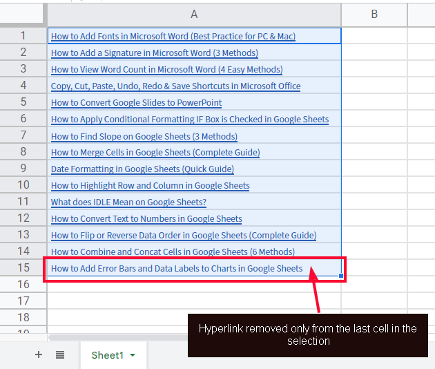
This is the quickest method to remove a hyperlink, but what if I need to remove all the hyperlinks in one click? No, this method does not remove all the hyperlinks together, if I select all and then do the same, so it will only remove the hyperlink for the last item in the selection
Step 5
Let’s try removing all the hyperlinks by selecting the entire list
Step 6
You can see only the last hyperlink is removed and the rest are still there
There is another easy method we will see in the next section.
Remove Hyperlinks in Google Sheets – using Right-click and Unlink
In this section, we will learn how to remove hyperlinks in google sheets by using right click and unlink method. This method is also very easy and has the power to remove all the hyperlinks in one click. So, I have the same data set and we will see how to remove all of them together.
Step 1
Select all the cells you want to remove hyperlinks from
Step 2
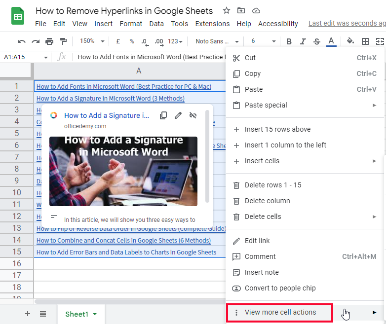
Right-click on any cell to open the options
Step 3
Go to ”view more cell actions”
Step 4
Remove link
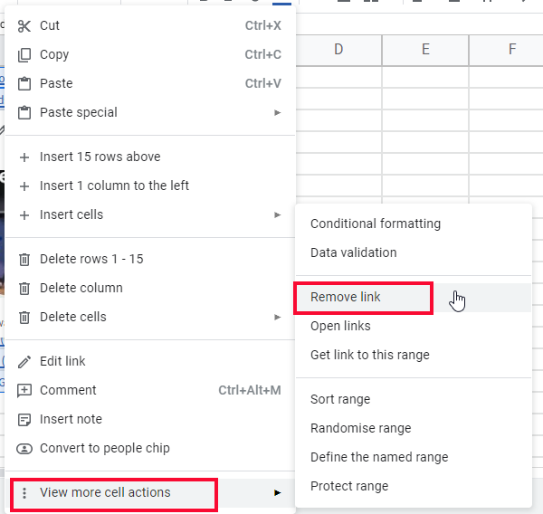
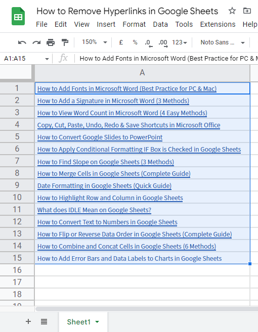
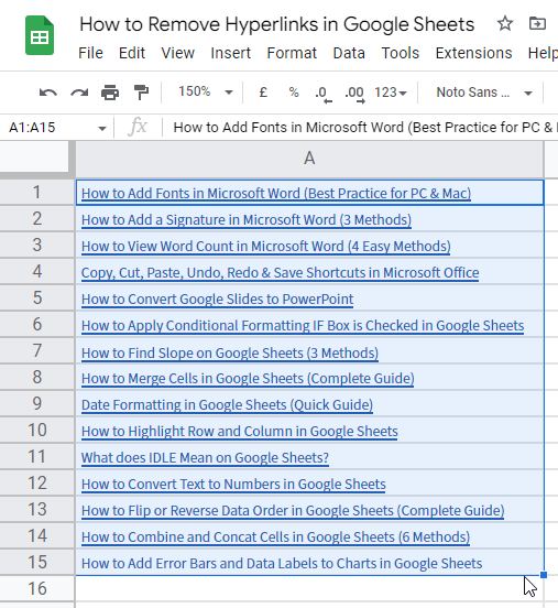
This instantly removes all the links of your selected cells and all the text will remain as normal text.
This is the fastest method if you want to remove hyperlinks from multiple cells and ranges.
We have more methods to remove hyperlinks, let’s see them below sections.
Remove Hyperlinks in Google Sheets – using Copy & Paste Special
In this section we will learn how to remove hyperlinks using a simple copy and paste special trick, this is the most used method by old google sheets users. This method also works for removing formulas. This method is simple, copy the content and paste it as values, then the links, and formula, will automatically be removed and the rest is only values, and this is what we want.
So I am using the same data set to show you how to remove hyperlinks using this method.
Step 1
Select all the data you want to remove hyperlinks from
Step 2
Copy the data (CTRL is the shortcut) or you can right-click and then click on the copy button
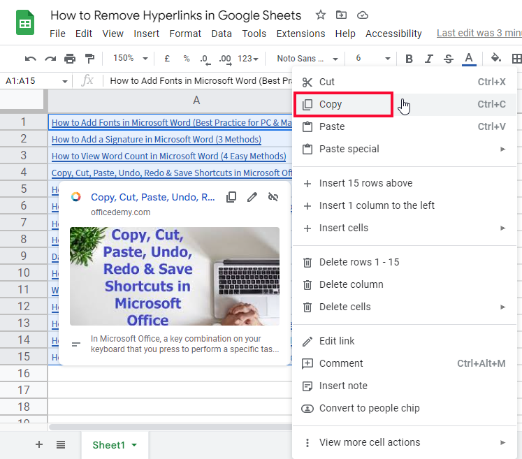
Note: Now you can paste them into the same position to replace the links with values, or you can paste them to another location to get a copy for values only.
Step 3
Go to the position where you want to paste and right click
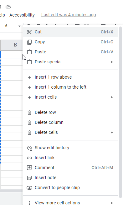
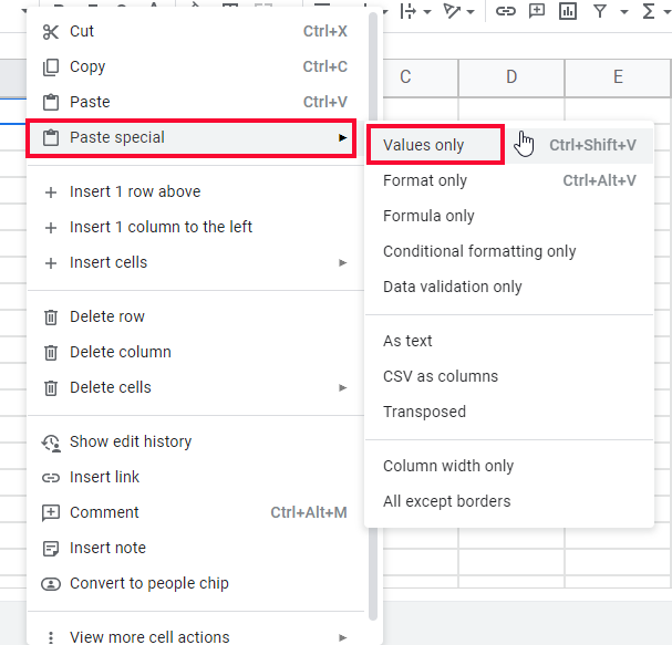
Step 4
Go to Paste special > Values only (Ctrl + Shift + V is the shortcut)
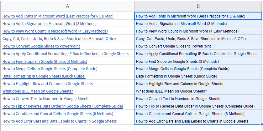
Step 5
Hyperlinks are removed, you can see your links are pasted as values
When making a copy of your links as values, you might be thinking that what if you have some changes in your original links, will they reflect in the copy of the values? No, they will not reflect, the paste method is not dynamic.
But, don’t worry, we have another method to remove hyperlinks that is capable of keeping the live changes in your original data, yes you can get the links as values, and then you will get the automatic changes if made in the original links.
Let’s see this method in the below section.
Remove Hyperlinks in Google Sheets – Using a Custom & formula
In this section, we will learn how to remove hyperlinks in google sheets using a custom & formula. This method is the best one to use when you want to have real-time changes, so it’s the only method that can give you live changes and updates of data when a change is made in the original link. Let’s see how it’s done.
I have the same dataset; I will use this formula in the adjacent column and will get the values of the links in a new column.
Step 1
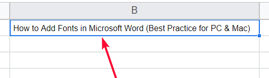
Start writing the formula in the cell you want to get the links as values
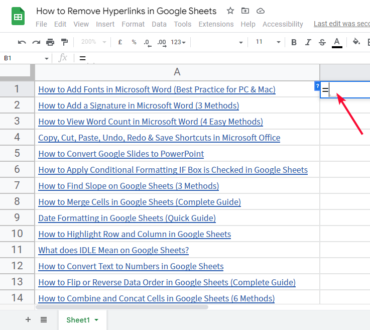
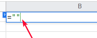
Step 2
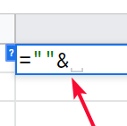
The formula can be hard to understand but it’s very short and straightforward
=””$cell_reference
Step 3
The cell reference is the cell in which you have your link written
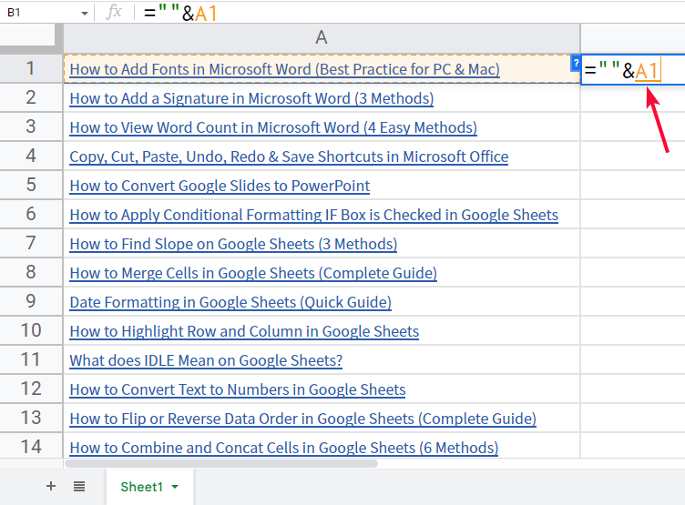
Step 4
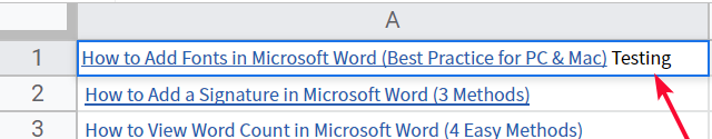
Press Enter key and you will get the value of the link
Step 5
If you have more links, you can simply drag the formula in the below cells, or double-click on the fill handle to fill the rest of the column

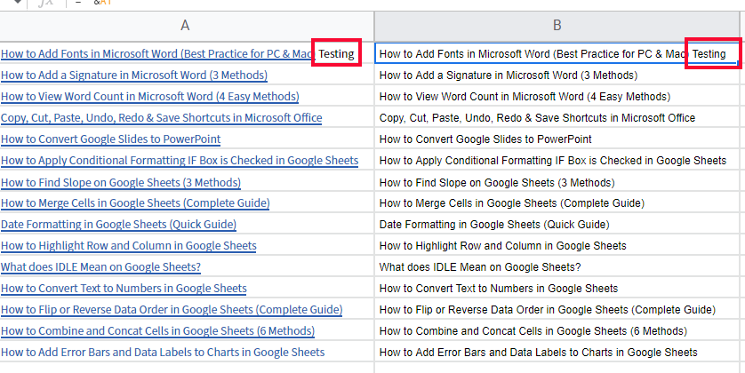
Since this method is dynamic, let’s test it out by making some changes to the original link
Step 6
Making some changes to the link
Step 7
You can see the change is automatically reflected here
This is how this method works, I hope you have understood and learned all the above methods, and now you remove hyperlinks using any of these.
I hope you find this article helpful.
For better practice, you can get a free copy of the workbook below.
Download/Copy Google Sheets Workbook
Important Notes
- The first method in which we removed the link from the icon in the link dialogue box, this method will not work until you select the cell and then click on the icon
- In the second method in which we removed all the hyperlinks together by right-click method, in this method, the remove link option can also be on the first window, and not on the “view more cell actions”
- The third method paste as values can use to paste on a new position and also be pasted on the same position to replace the links with values
- The fourth method, the custom formula method gives us dynamic behavior by which we can have the real-time changes and updates that are made on the original links. If you want to stop them you can use the third method, copy all the values generated by the formula, and paste.
Conclusion
In this tutorial, we learned how to remove hyperlinks in google sheets. We have discussed four useful methods, that can be used to remove hyperlinks in google sheets. We first discussed what are hyperlinks and why we need to remove them, then we saw four useful ways and implemented them on a sample link list. I hope you have gone through all the methods and learned how to use them practically on your data.
That is all from how to remove hyperlinks in google sheets. I will see you next time with another helpful tutorial. Keep learning with our spreadsheet templates provided in every article. Thank you so much and have a nice day.


