How to Strikethrough on Google Sheets [4 Methods]

In this article, we are going to learn different ways and methods of applying strikethrough formatting in Google Sheets. It is a rarely used function but very useful for most applications like Google Docs or MS Word. Keep on reading to discover strikethrough formatting options in Google Sheets and get ready to use this formatting in your spreadsheet as well.

What is Strikethrough?

Strikethrough is primarily used to highlight text that is incorrect or needs to be deleted without actually removing it. It is also used to indicate some tasks that have been completed. It is a character format and style added to a text as a continuous horizontal line that passes through the middle of the text indicating the removal of some error or mistake.

Nowadays it becomes a way of saying something without really saying it to express our opinion on any subject which can be different from the fact but known by everyone. We can use strikethrough to draw attention to the specific area. People are also using it for ironic humor in online informal conversations.

Why use Strikethrough on Google Sheets

A strikethrough is a useful tool and function. Through this article, you will explore the advantages of this feature and find its significance and importance. For example, sometimes when we are making a checklist of tasks, we want to cross out those tasks which have been completed.

Strikethrough doesn’t just imply a revision of errors but it can also be used to deliberately indicate changes as you often note it’s used during online shopping when some product or item is put on sale or discount, they cannot remove its original price but it needs to be cut down to write a new price of that product after discount.

It is also useful to highlight invalid and outdated content. Likewise, we can have many other possible purposes where we need to use strikethrough formatting.

How to Strikethrough on Google Sheets

In Google Sheets, there is not a single way to apply strikethrough although for your comfort there are four easy methods to apply strikethrough. It depends on you which method you prefer according to your comfort zone.

Following are the three simple ways to apply strikethrough formatting in your Google Spreadsheet.

1. Using a Keyboard Shortcut
2. Using Strikethrough Option from the Toolbar
3. Using Strikethrough Option from the Menu
4. Add Strikethrough by Conditional formatting

Now we will find the step-by-step procedure of each method of how to apply strikethrough formatting in Google Sheets. So let’s get started!

Strikethrough on Google Sheets – Using a Keyboard Shortcut

This is a very easy and quick method to apply strikethrough formatting in your spreadsheet consisting of only a few clicks which are shown below.

Step 1

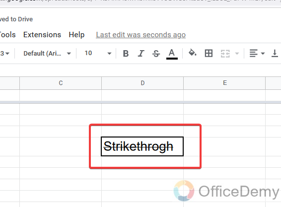
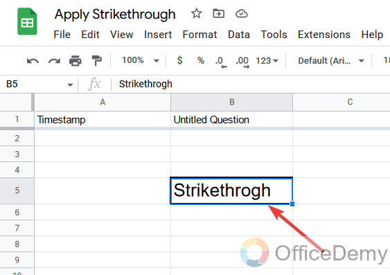
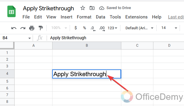
First, you need to select the cell or number of cells in which you want to use strikethrough formatting.

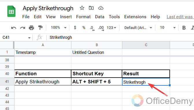
Step 2

In the second step, you are ready to use the shortcut key which is ALT + SHIFT + 5, and get your work done by pressing these keys together at the same time.

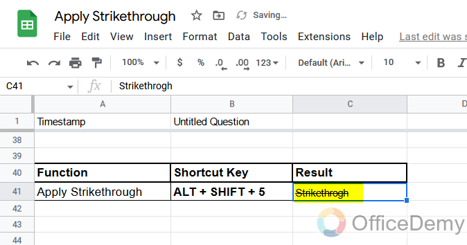
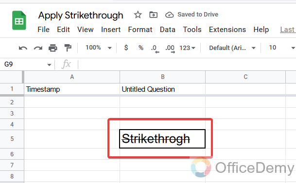
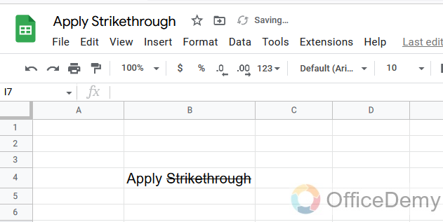
As you may see the text has been applied strikethrough.

Note that this shortcut key can also be used in the same manner as mentioned above to remove strikethrough formatting in your spreadsheet.

Strikethrough on Google Sheets – Using Strikethrough Option from the Toolbar

Another way to have your work done is using the strikethrough option from the toolbar which requires just a click and you will see the result in a blink of an eye. Following are the steps of this method.

Step 1

First, you need to select the cell or number of cells in which you want to use strikethrough formatting.

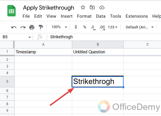
Step 2

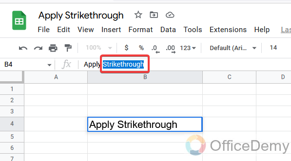
After selection, find the strikethrough button in the toolbar at the front. As shown in the image

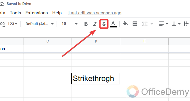
Step 3

Just click on this button to apply strikethrough the selected text or cell. As you may see below.

Note that this method can also be used in the same manner as mentioned above to remove strikethrough formatting in your spreadsheet.

Strikethrough on Google Sheets – Using Strikethrough Option from the Menu Bar

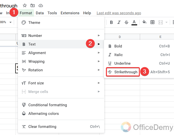
Step 1

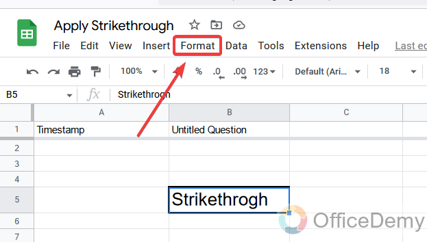
First, you need to select the cell or number of cells in which you want to use strikethrough formatting.

Step 2

Now, in the menu bar you have the “Format” option, Click on it to open a drop-down menu.

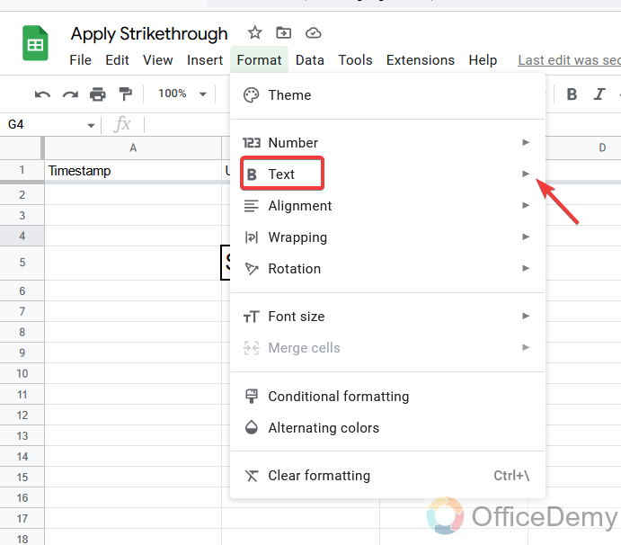
Step 3

In the drop-down menu, you will find “Text”. Click on it to open it again in a drop-down menu.

Step 4

In this menu, you will find the “Strikethrough” button from which you may apply strikethrough to your text with one click only.

Step 5

The result is in front of you as a click.

Yes, the previous two methods are more convenient to use but still, this method is included just to show you all the possible ways to do the same task i.e. applying Strikethrough formatting in Google Sheets. And like other methods, this method can also be used in the same manner as mentioned above to remove strikethrough formatting in your spreadsheet.

Now you have learned all the methods of applying strikethrough formatting and you are ready to apply strikethrough on the complete text written in a cell or number of cells.

Strikethrough on Google Sheets – Using Conditional Formatting

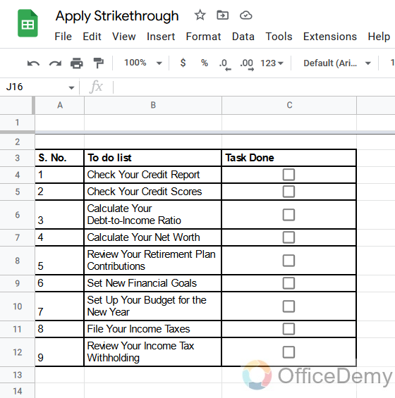
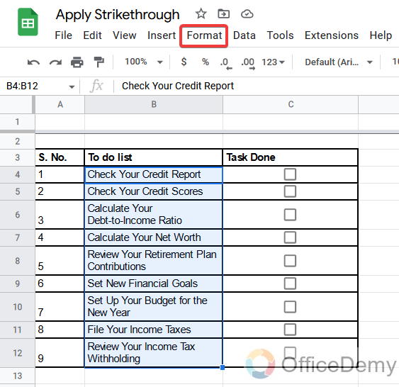
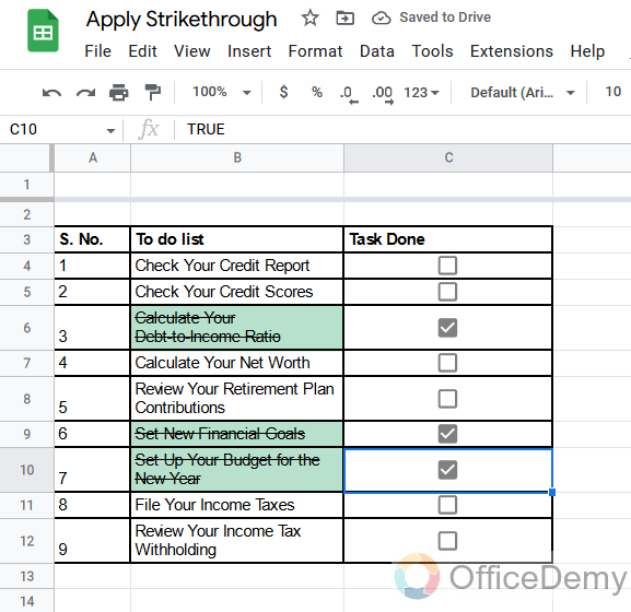
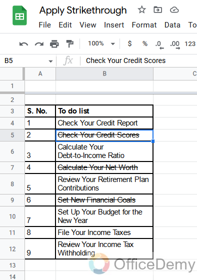
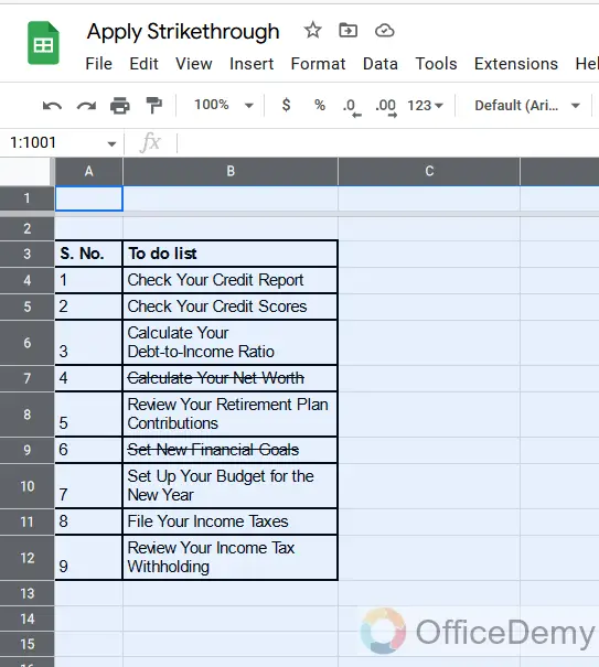
Let’s suppose you have created a to-do list in Google Spreadsheet and you want to apply strikethrough automatically whenever you mark them checked. This could be done by using conditional formatting. Here is an example of a to-do list. You can see several tasks in the picture on which we are going to apply strikethrough.

Following are the steps for applying strikethrough formatting conditionally in Google Sheets.

Step 1

Let’s suppose we have such type of data on a to-do list.

Step 2

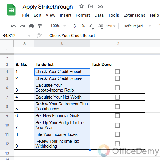
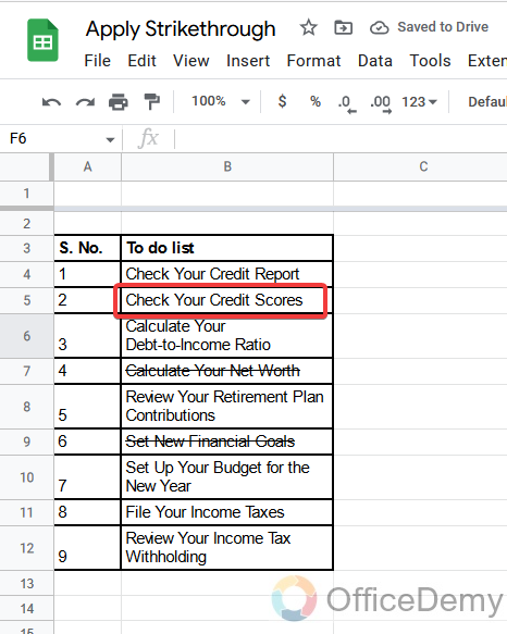
First, select the range of cells where you want to apply conditional formatting. In our example, we will select cells B4 to B12.

Step 3

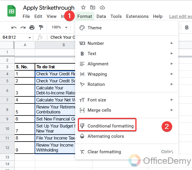
From the main menu, find and select the “Format” tab.

Step 4

From a drop-down that appears, navigate to “Conditional formatting”.

Step 5

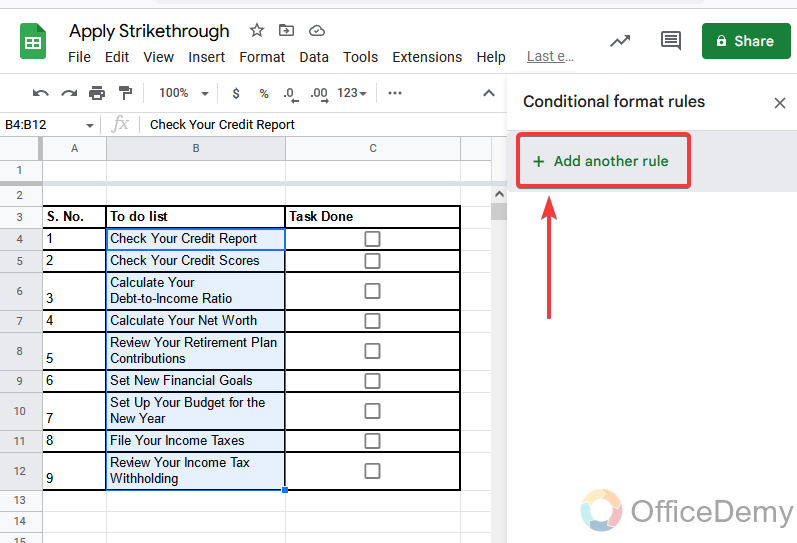
A new window will open on the right side of the sheet, where you will make new conditional formatting by clicking on “Add another rule”.

Step 6

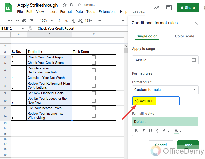
Here as the range is selected now, you will need to change “Format cell if…” to “Custom formula is”.

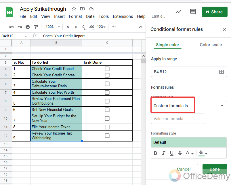
Step 7

Write down the conditional rule in the space below. According to our sample data, the formula will be written as “=$C4=TRUE”. In this way, it will apply this formatting if we mark the checkboxes present in Column C.

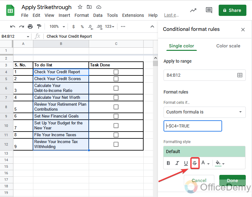
Step 8

Now look under the “Formatting style” and select the “Strikethrough format” option.

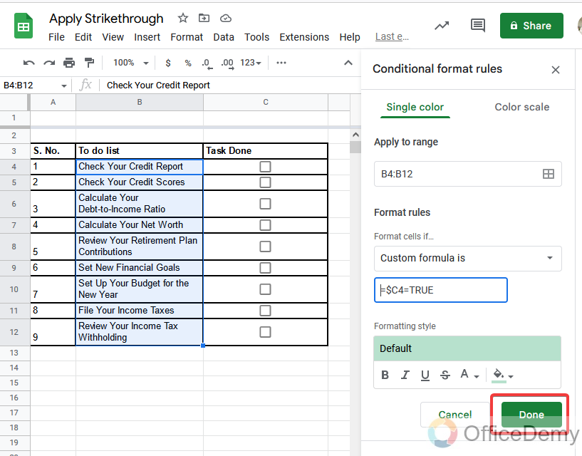
Step 9

You are almost done finally click on “Done” to complete the process.

Step 10

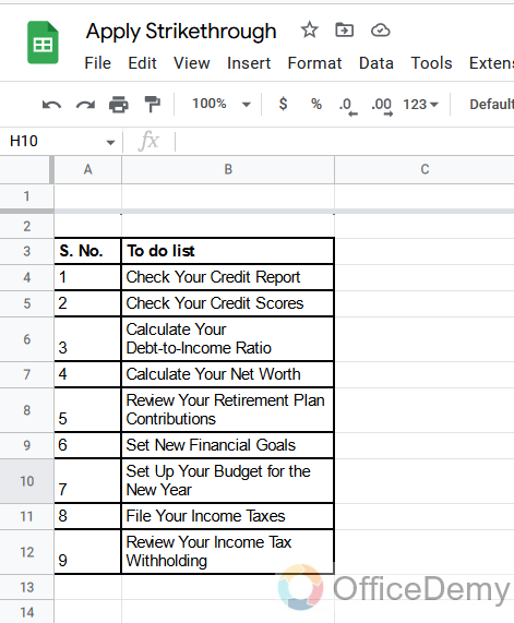
Now if you mark the checkbox you will see the strikethrough appears automatically for that task.

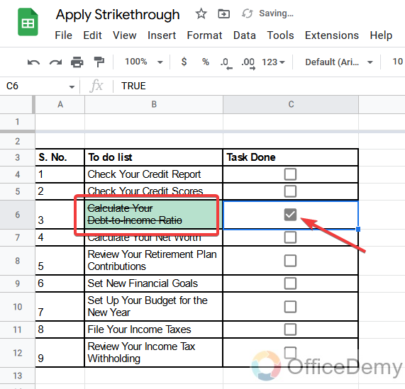
Step 11

As we have applied formatting to the whole list so when you checked any of them you will see the strikethrough appears. As you may see below

Frequently Asked Questions

How to apply strikethrough formatting on a part of the text written in a cell?

Here you will get your answer on how to apply strikethrough formatting just on a part of the text. Follow these steps to avoid strikethrough formatting on a complete cell.

Step 1

First, you need to get into the editing mode by double-clicking the cell.

Step 2

Now select the part of the text written in the cell on which you want to apply strikethrough formatting

Step 3

In the toolbar, click on the strikethrough icon (or press the shortcut key ALT + SHIFT + 5 or select the strikethrough option from the format tab in the main menu).

You can also apply bold, italic, and underline tools to your text in a similar way.

How to remove Strikethrough formatting from a cell or number of cells?

The same methods which are explained earlier to add strikethrough are also used to remove strikethrough i.e.

Step 1

Press right-click to select the cell in which you want to remove the strikethrough.

Step 2

In the toolbar, click on the strikethrough icon (or press the shortcut key ALT + SHIFT + 5 or select the strikethrough option from the format tab in the main menu).

If you have applied strikethrough randomly on multiple cells and now want to remove this formatting from all of them, follow these steps.

Step 1

Select the entire spreadsheet by clicking on this gray box present at the top left corner of your sheet.

Step 2

In the toolbar, click on the strikethrough icon (or press the shortcut key ALT + SHIFT + 5 or select the strikethrough option from the format tab in the main menu).

It will remove the strikethrough wherever you have applied it earlier without affecting the remaining cells.

Conclusion

In this article, we have covered different methods of how to apply strikethrough in Google Sheets. You can use the keyboard shortcut and alternatively go for options in the toolbar or menu to apply strikethrough to your text in Google Sheets. It works like a toggle button which means you can get your text with the original formatting again and easily remove the strikethrough if you use the strikethrough option twice. I hope all the methods are easy to understand and will help you to practically apply them in your Google Sheets.

If you find this article helpful, I’ll recommend you to come again and also learn about other features of Google Sheets with Office Demy. Thank you!