
To Use IFNA Function in Google Sheets
- Use =IFNA(value, “Custom text“).
- Replace “value” with the function or value you want to check for #N/A error.
- If #N/A error occurs, it displays the custom text.
OR
- Use =IFNA(VLOOKUP(D1,$A$1:$B$4,2,FALSE), “Value not found“).
- VLOOKUP searches for a value in a range.
- If not found, it returns #N/A error, and IFNA shows the custom message.
OR
- When #N/A error occurs, use =IFNA(VLOOKUP(D1,$A$1:$B$4,2,FALSE), VLOOKUP(D1, AnotherSheet!$A$1:$B$4,2,FALSE)).
- This searches for the value on another sheet if not found on the first.
OR
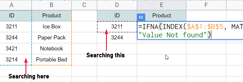
- Use =IFNA(INDEX(A1:B5, MATCH(D2, A1:A5, 0)), “Value Not found“).
- INDEX MATCH is similar to VLOOKUP but may return #N/A >IFNA displays a custom message instead.
Hello, welcome to the IFNA Google Sheets tutorial, in this article, we will learn how to use the IFNA function in Google Sheets.
IFNA function is one of the errors handling functions in google sheets that deal only with the #N/A error. Now #N/A error occurs when a search key is not found. It returned my many functions such as VLOOKUP, HLOOKUP, IF, SUMIF, etc.
The functions used for searching a key can return a #N/A error when that item is not found, now we can handle #N/A errors by using the IFNA function and we can tell google sheets to print a specific string or text when there is an #N/A error. It helps us keep the sheets clean and understandable for every user.
IFNA Function in Google Sheets
We use a lot of functions in our big google sheets file, we have a lot of data and we often need to search the data in certain ways to get the results or to verify whether the value is present or not. There are many reasons we need to use search keys in a column or a range. We generally use VLOOKUP, HLOOKUP, or IF to search for the key in google sheets. This function returns the answer or returns the #N/A error when the search key is not found.
The #N/A error is very bad in the sheets, and if we don’t use error handling our google sheets file looks pretty bad and seems to have a lot of mistakes. This is why we have error handling functions like IFNA, we need to learn them to control the error messages and to print more meaningful and clean messages when the #N/A error encounters.
- For #N/A error handling in google sheets
- To maintain the aesthetics of our file
- To improve the readability of the data for new users
How to Use IFNA Function in Google Sheets
To learn how to use the IFNA function in google sheets, we have a set of steps called a method. we will learn three different use cases to use IFNA Function, we all also see some theoretical concepts and also little about other similar errors.
First, here we have three use cases to use the IFNA function, Let’s start with the first one.
How to Use IFNA Function in Google Sheets with VLOOKUP Function
In this section, we will learn how to use the IFNA function in Google sheets with VLOOKUP Function. For this first, let’s take a quick look at VLOOKUP Function.
Syntax
=VLOOKUP(D1,$A$1:$B$4,2,FALSE)
VLOOKUP function means Vertical lookup for the search key that is provided by users in the parentheses.
Here,
D1: is the search key we want to lookup
$A$1: $B$4: is the range of the data written in $ Notation, where we want to search the search key
2: is the column number (column 2 = column B), which values we want to get against the search key
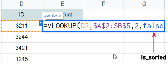
FALSE: is the parameter to is-sorted, which means the range is not sorted
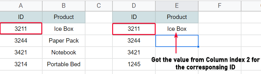
The above VLOOKUP function will search the key (D1) in the range A1:B4, and return the values corresponding value of the D1 in column 2 if found, if not found; it will return a #N/A error which means that the key (D1) was not found.
Now, for error handling, we will use IFNA along with VLOOKUP to print a meaningful message only when there is an #N/A error, if an #N/A error does not occur, you will not see any effect of the IFNA function.
Let’s practically see this example in the steps below.
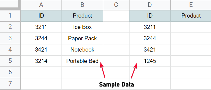
Step 1
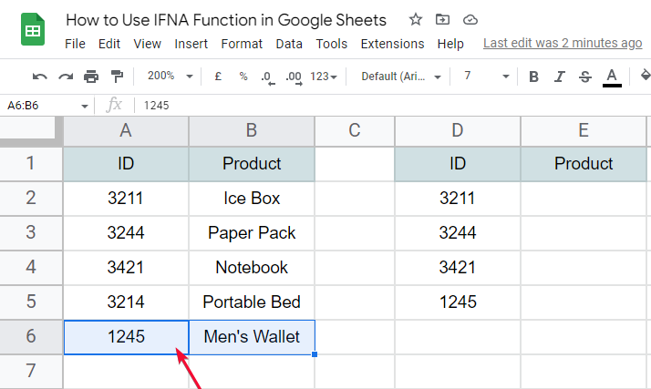
Make similar sample data to follow this example
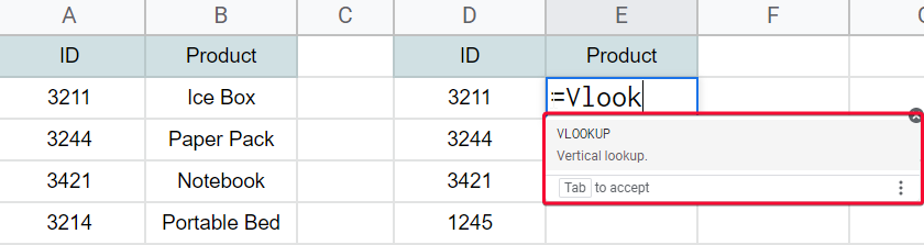
Step 2
Write the VLOOKUP function
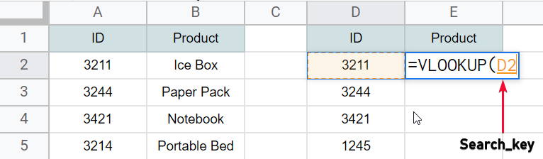
Step 3
Pass the first parameter (search-key)
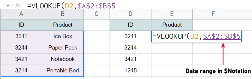
Step 4
Pass the second parameter (data range in $ notation)
Step 5
Pass the Index number (column number from which you want to retrieve the corresponding values)
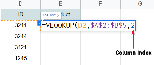
Step 6
Pass False for unsorted range (True for sorted range)
Step 7
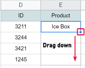
Hit Enter and see the result, drag for the entire column
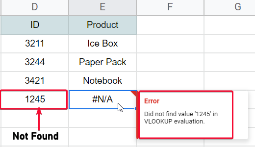
Step 8
I got a #N/A error because a key is not found
Step 9
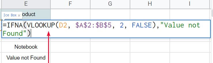
Adding the IFNA function in the starting, and making the VLOOKUP formula the first parameter of the IFNA function.
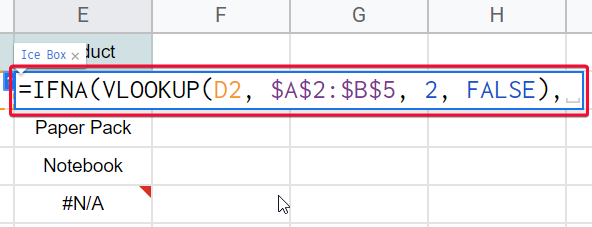
Step 10
Add a comma, and pass the second parameter (text in double-quotes that should be appeared whenever an #N/A error occurs)
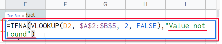
Step 11
The overall formula will be
=IFNA(VLOOKUP(D1,$A$1:$B$4,2,FALSE),(“Value not found”))
Step 12
Now you can see the custom text is appearing instead of an IFNA error.
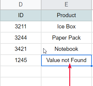
This is how to use the IFNA function in Google sheets with VLOOKUP Function
How to Use IFNA Function in Google Sheets with VLOOKUP Function to Search Other Sheets When #N/A Error Encountered
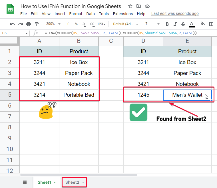
In this section, we will see how to use the IFNA function to only print a custom text when an #N/A error is encountered but to perform another search on other ranges or even other sheets when an #N/A error is encountered, let’s say we have the same data as used in the previous section, and we have one search key that is not found, but we have another sheet and in that sheet, we have similar data where the unmatched key could exist, so what we do, we tell google sheets to perform a search on our other sheet when the search key is not found in the existing range. Let’s understand it step-by-step with an example
Step 1
Similar data set in another sheet
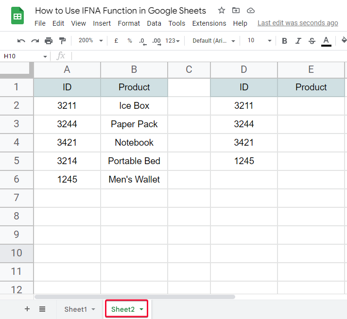
Step 2
In another sheet, we have the search key that was not found in the previous sheet.
Step 3
Now come to the old formula in sheet 1
Step 4
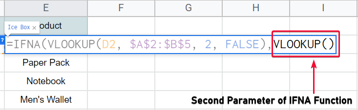
As the second parameter of the IFNA function, remove the custom text, and add another VLOOKUP function
Step 5
Define the parameters sheet and range
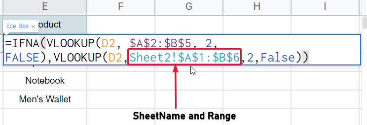
Step 6
Now hit Enter key and you can see the unmatched key is found on another sheet and it’s showing the key instead of an #N/A error or a custom message.
This is how we can further take advantage of the IFNA function in google sheets by passing another range or sheet to research the key.
How to Use IFNA Function in Google Sheets – Difference Between IFNA and IFERROR
Now IFNA and IFERROR are different in the sense that if error directly handles the error regardless of its type. IFERROR can be used with certain functions to do something instead of throwing an error (any kind of error), while the IFNA function is solely for the #N/A error, #N/A error mostly occurs when we use searching Functions like IF, IFS, SUMIFS, VLOOKUP, HLOOKUP, etc. So, keep in mind the IFNA is only for #N/A error and IFERROR is for general purpose regardless of error type.
Syntax
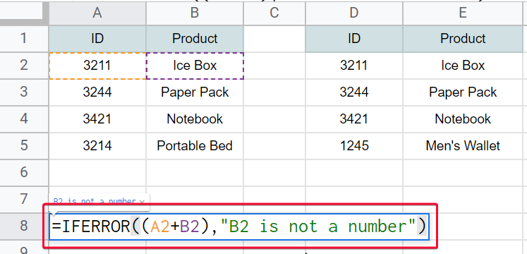
IFERROR(value,value_if_error)
Example of IFERROR
How to Use IFNA Function in Google Sheets – With INDEX MATCH Function
In this section, we will learn how to use IFNA Function in Google sheets with the INDEX MATCH Function. INDEX Function works similarly to VLOOKUP Function, it looks for a value in a specified range of cells and returns the matched results, and if not found it returns an #N/A error just like VLOOKUP.
Syntax
MATCH(lookup_value, lookup_array, [match_type])
Here,
lookup_value – the number or text want to search
lookup_array – the range in which we search the value
match_type – specifies whether to return an absolute match or partial matches as well
Let’s see how it works with a Step-By-Step procedure
We are using the same example so I will skip some repeating steps
Step 1
Write the formula
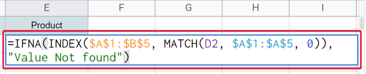
=IFNA(INDEX(A1:B5, MATCH(D2, A1:A5, 0)), “Value Not found”)
Step 2
Similar pattern as we saw in VLOOKUP
Step 3
Hit enter, drag the formula, and you can see it will show “Value not Found for every unmatched search key”
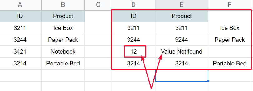
This is how to use IFNA Function in Google sheets with the INDEX MATCH Function and get the desired result instead of an ugly #N/A error.
Download/Copy Google Sheets Workbook
Notes
- The second parameter is optional if you pass only the VLOOKUP or any other function, so when the #N/A error comes, I will return the empty string. Since an empty string is not mean we also use the second parameter.
- IFNA only deals with #N/A Errors, it will not work with any other errors like #DIV/0 error, #REF error, etc.
- IFNA and ISNA are different functions IFNA is used when we want to perform a certain action when an #N/A error is encountered and the ISNA function is only used to evaluate if a cell contains a #N/A error.
- IFNA takes two arguments, the first is the function, and the second is the action to be performed when an #N/A error is encountered.
- ISNA function takes only one argument that is similar to the second argument of the IFNA function, it only takes what to do when an #N/A error is encountered, and it returns TRUE or FALSE if the cell contains an #N/A error or does not contain an #N/A error respectively.
Conclusion
So today we learned a very useful error handling Function IFNA, we learned how to use IFNA Function in Google Sheets to deal with #N/A error, we have seen multiple use cases of the IFNA function and tried to cover the basic theoretical principles about it, I also tried to clear the common misunderstanding regarding IFNA and IFERROR, and also IFNA and ISNA. So, after this article, you will be easily managing your #N/A error smartly with custom text or any other action be performed when an #N/A error occurs. We have seen IFNA with VLOOKUP, with VLOOKUP on multiple sheets, we saw IFERROR, we saw IFNA with MATCH INDEX Function and we also discussed some general important points in the NOTES section. That all form how to use IFNA Function in Google Sheets, see you soon with another tutorial till then take care and keep learning with Office Demy.


