How to use OFFSET Function in Google Sheets [Guide 2023]

In this article, we will learn how to use OFFSET function in google sheets. The OFFSET function is an underrated function in google sheets, since it’s a bit tricky sometimes users avoid it. But trust me it is a great function with great features and it’s so powerful when it comes to cell references. The OFFSET function is used to refer to a cell without the cell address, it’s just another way to call cell references to use in the formula or to get the values of the cell(s).

Now you will be thinking, how can we call a cell without its reference? Yeah, there is a way we can use as per the OFFSET of a cell, and based on the location we can get the cell values using the OFFSET function. We will see how to use this function and we will see some useful applications of this function when working with google sheets.

Why we use OFFSET Function in Google Sheets

We normally work with cell references, but there can be certain situations where we don’t want or can not use the cell references to refer to a cell or range, or other reasons can be, we know there will be a lot of change in the cell references so we can use the OFFSET function to call cells in these situations. Now you may think why do we need OFFSET when we can use absolute and relative cell references?

We have situations where the absolute references along with some functions do not match the actual range when there is a row or column added to last or on the start point. In this situation, we will easily lose our cell references even if they are absolute. So, to deal with such cases we can use the OFFSET function at its best. We can also use this function casually to refer to cells and ranges. Let’s see the usage and benefits of this Function in google sheets.

How to use OFFSET Function in Google Sheets

From here, we will learn the step-by-step procedure to understand the OFFSET function first, we will see some examples of it, and then we will move to some practical examples. Let’s start with the syntax.

Syntax of OFFSET Function

=OFFSET(reference, rows, cols, [height], [width])

Here,

1. Reference: is the cell where you want to get the result and from where you are measuring your OFFSET. It is normally a cell in which we are using the OFFSET function. We can measure the OFFSET from the current cell too.
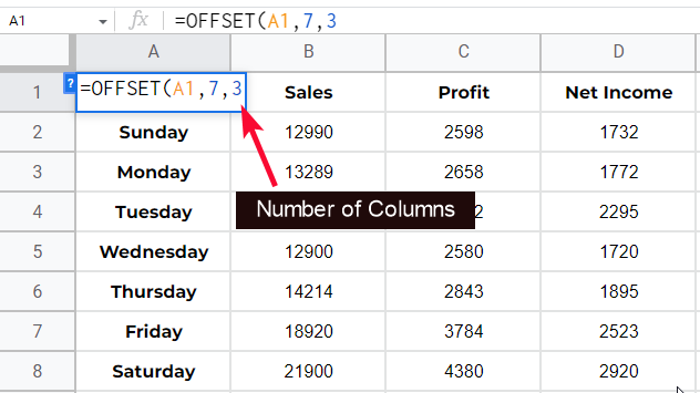
2. rows: are the number of rows away from your reference cell, it is passed in numbers such as 3
3. cols: are the number of columns away from your reference cell, it is also passed in numbers such as 2
4. height: is the height (number of rows) from your cell that has been selected by the above parameters, it is used when we want to refer to an array.
5. width: is the width (number of columns) from your cell that has been selected by the previous parameter, it’s also used only with the last (height) parameter.

Height and Width are the optional arguments. They can be omitted; they are only used when we need to return an array instead of a cell.

Sample Syntax

=OFFSET(A1, 2, 3, 3, 2)

OFFSET Function in Google Sheets – Refer to a single cell

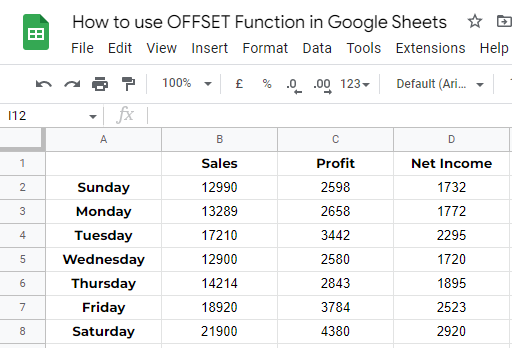
In this section, we will learn how to use OFFSET function in google sheets to refer to a single cell in google sheets. We have a sample dataset for this example we will see how (without using cell references) we can refer to a cell and get its value into another cell.

Step 1

Sample data

Step 2

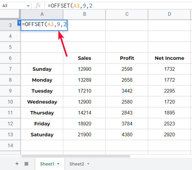
OFFSET function in cell A1

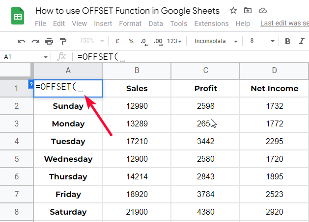
Step 3

Pass the first argument

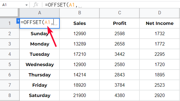
Step 4

Pass the second argument

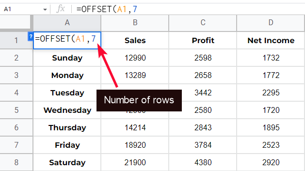
Step 5

Pass the third argument

Step 6

Hit Enter key and you’re done.

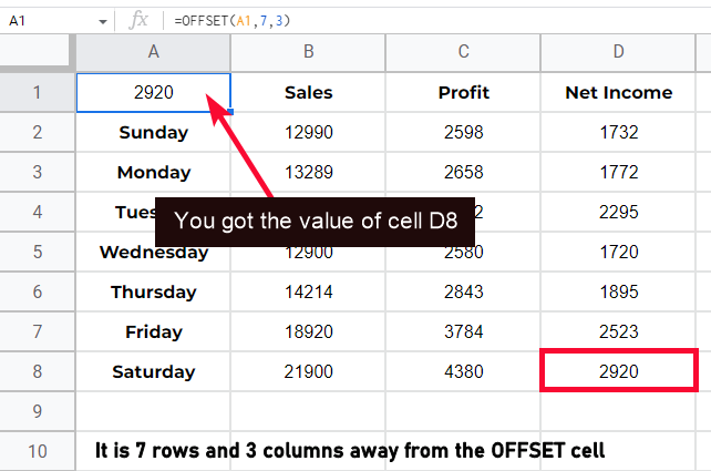
You see how we got the cell value using OFFSET, this is the power of OFFSET

Explanation of the above Example

Here the OFFSET function will look for a cell that is N rows (second parameter) away from the A1, after finding a cell, it will save the row number and look for the column which is N columns (third parameter) away from the A1. This is how it will get one cell and will return the cell value in cell A1.

OFFSET Function in Google Sheets – Refer an Array

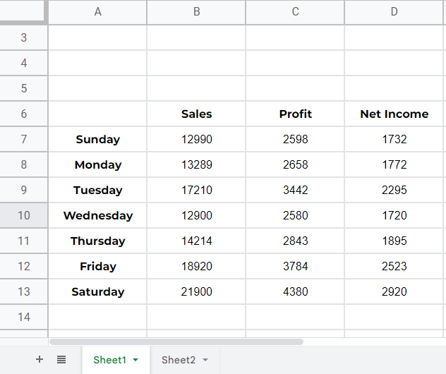
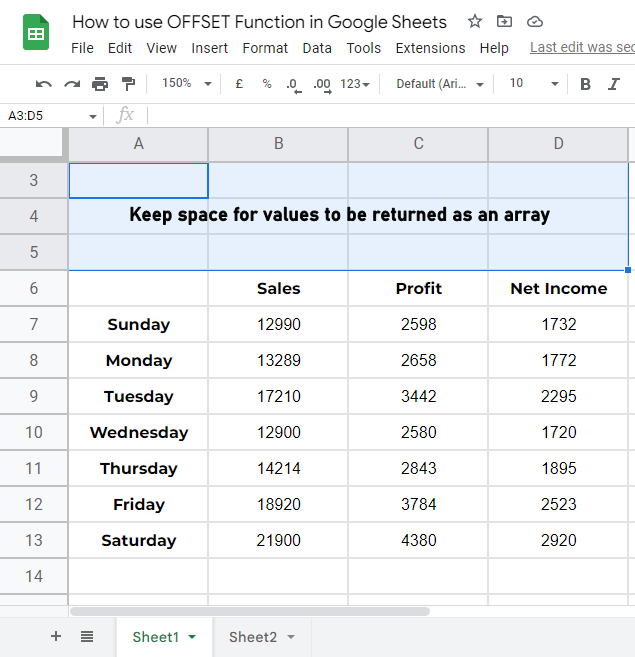
In this section, we will learn how to use OFFSET function in google sheets to refer to an array of cells. We will refer to an array and will return this array as we return using an ARRAYFORMULA. Note that, you must have empty cells around your OFFSET cell (A1) to get the result in return, otherwise the function will return an error with a message that there is no space to expand the formula.

Step 1

The same data set

Step 2

Spaces for the values to be returned

Step 3

Passing first, second, and third parameters.

Step 4

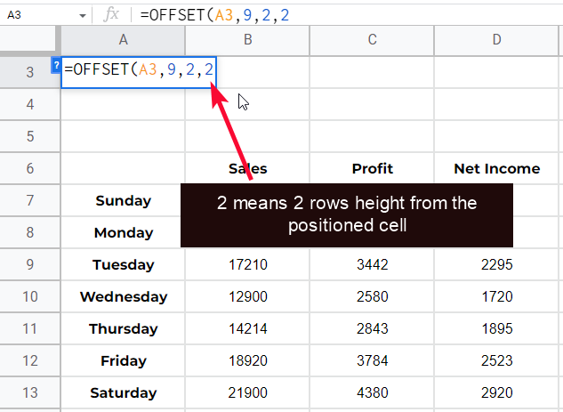
Passing the fourth parameter (height)

Step 5

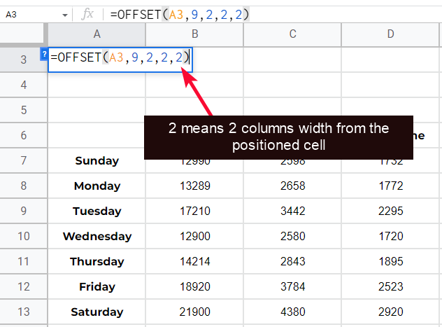
Passing the fourth parameter (width)

Step 6

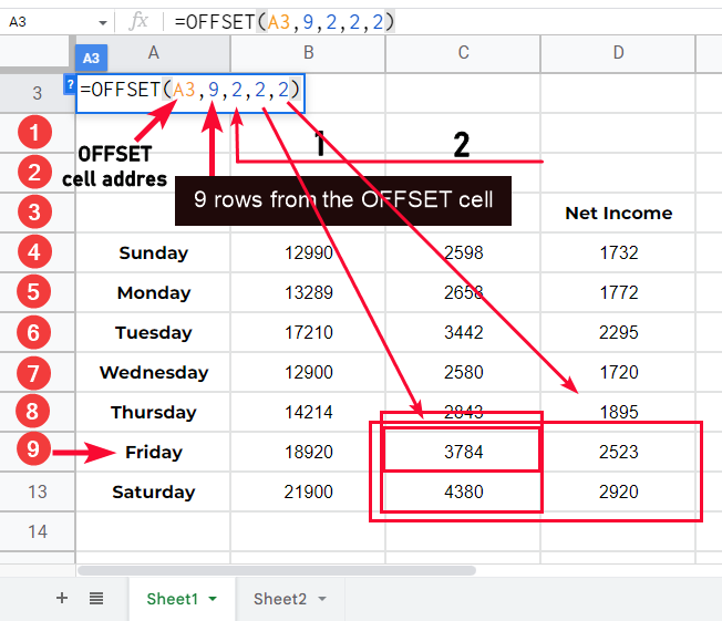
See below the projected result for your understanding

Step 7

Press Enter key, and you’re done

This is how you can return an array using the OFFSET function in google sheets.

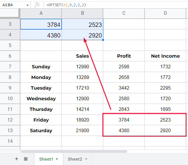
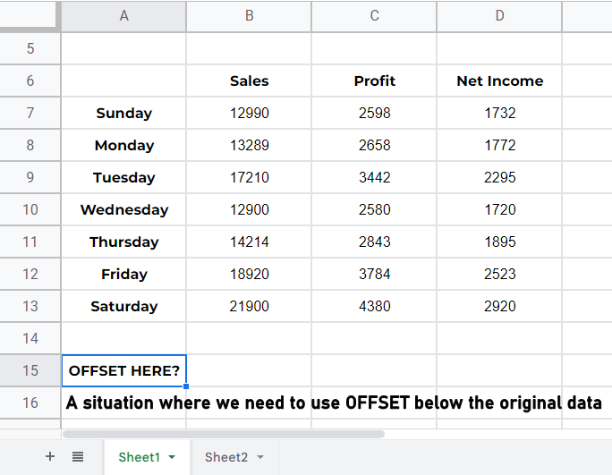
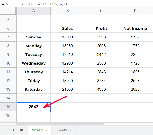
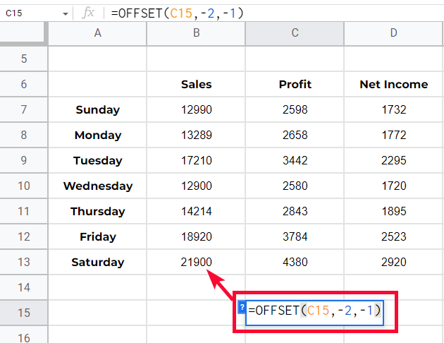
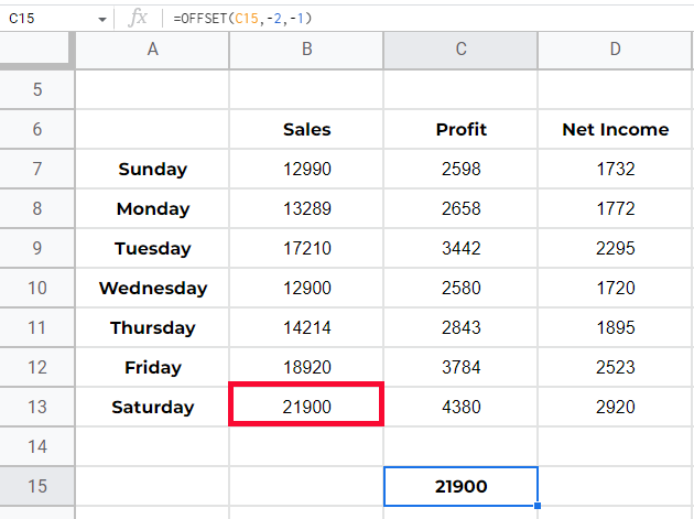
Refer Cells when the OFFSET Cell is Below in Google Sheets

How can you refer to a cell when your OFFSET cell is below the original data? It’s very very simple you can use negative values as well. So, in a situation where your OFFSET cell is below, right, left, or anywhere from your data you can use negative values, negative and positive together (negative on each axis, and positive on the other).

Step 1

Sample situation

Step 2

In the below cell start writing the OFFSET function

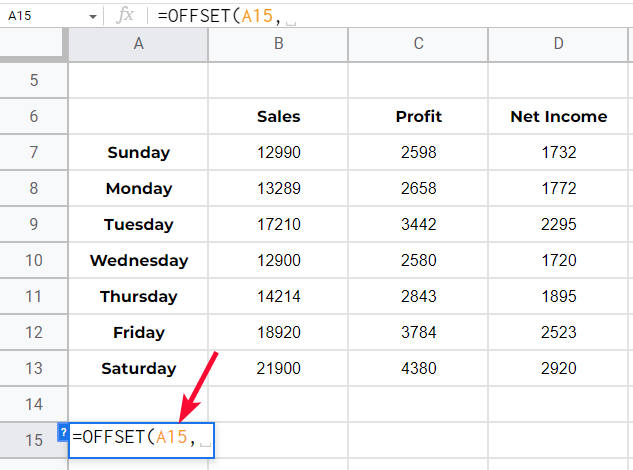
Step 3

Now you can count negatively to refer to a row

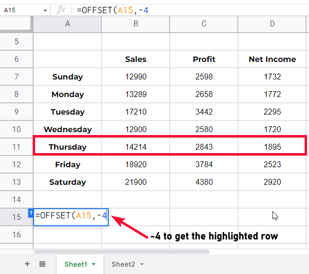
Step 4

The formula is completed, press Enter key to see the result

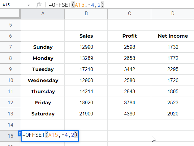
Now a similar condition for a negative value in for row as well as column

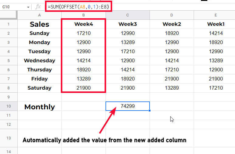
OFFSET Function in Google Sheets – With SUM Function

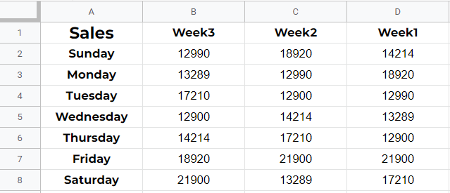
In this section, we will learn how to use OFFSET function in google sheets along with the SUM function. Now you can say what’s the need to use these functions. we can use SUM with direct cell references. Well, I will show you the answer to this question in the below example. So, let’s move forward for now.

Step 1

Sample data

Step 2

Calculating SUM using the SUM function

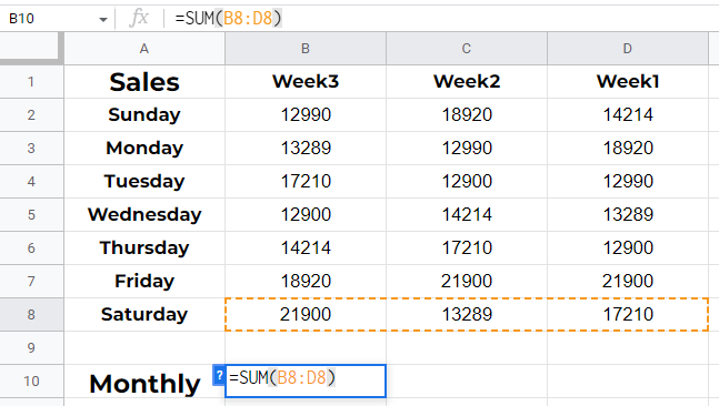
Step 3

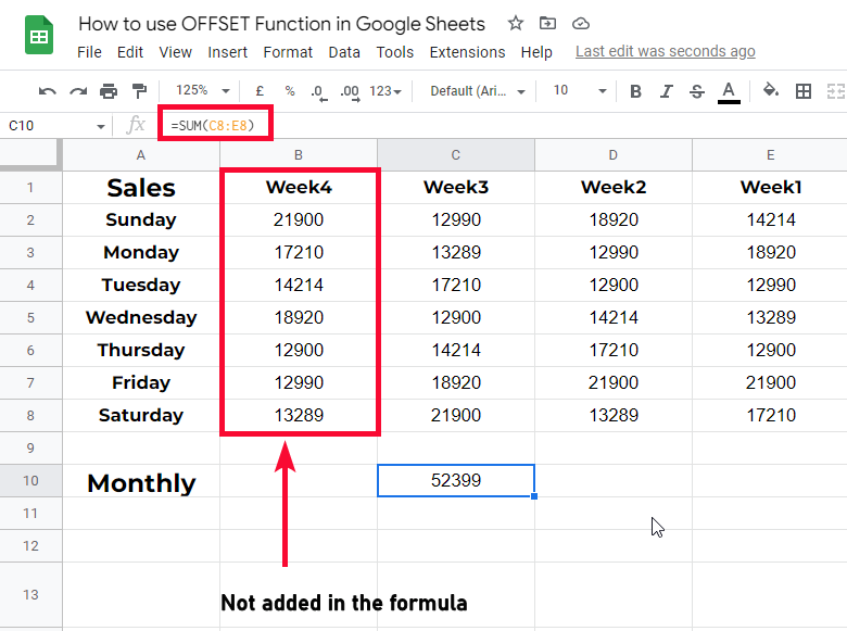
Adding a new column at the beginning

Step 4

You can see the formula is the same, and the new column is not being added to the SUM function.

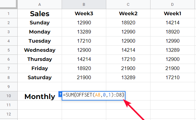
Now let’s do the same thing using SUM with OFFSET

Step 1

The formula will become

=SUM(OFFSET(A11,0,1):D11)

Now the above formula is different in the sense of logic building. Here we are not A8 inside the SUM function, instead, we are using an OFFSET logic to define that pick the value which is after the cell A8, make row distance 0, and column distance 1, and add along with the range F8, since we know that the columns can be added into starting or in the middle since the last column is total, so no column will be added after that, that’s why we hard-coded the last column as F8.

This is how we can use OFFSET with many more functions like AVERAGE, MATCH, INDEX, and many more as per need, the important thing is to understand the logic behind the OFFSET function.

Now the above formula can be moved to any cell in the sheet, it will still give you the same result and will be auto-updated when a column is added.

I hope you find this article helpful.

Download/Copy Google Sheets Workbook

Important Notes

Frequently Asked Questions

How to quickly use OFFSET function in google sheets?

OFFSET function can be used like another regular function, you need to know the syntax to use this function. We have a total of five arguments in this function the first is the cell reference of the cell from which we are measuring the OFFSET, the second is the number of rows away from the OFFSET cell, third is the number of columns away from the OFFSET cells. Then we have two optional arguments to return how many rows or columns, we pass a number to define height from which we can return multiple rows, then we define width to return multiple columns. This is how we can use the OFFSET function in google sheets.

What are the Similarities and Differences Between the QUERY and OFFSET Functions in Google Sheets?

The query function in google sheets and the offset function serve distinct purposes while having certain similarities. The query function allows you to extract specific data from a dataset based on given criteria. On the other hand, the offset function helps you to reference a cell or a range of cells that are a certain number of rows and columns away. Despite their disparities, both functions are valuable tools for manipulating and analyzing data in Google Sheets.

Can I Use the Linest Function in Combination with the Offset Function in Google Sheets?

Yes, you can definitely use the LINEST function in combination with the OFFSET function in Google Sheets. By using these two functions together, you can perform advanced data analysis and create dynamic formulas. The google sheets linest function helps to calculate the statistical line that best fits a given set of data, while the OFFSET function allows you to dynamically reference specific cells by adjusting the range based on a given offset value. Combine them to enhance your data manipulation capabilities in Google Sheets.

Conclusion

Wrapping up how to use OFFSET Function in google sheets. We have started with the basics and we learned about syntax, the syntax is itself very important because all the arguments look similar so we must need to understand the differences and the effect that come from each argument. We moved to some examples and how to return a cell value using OFFSET, then we saw how to return an array using OFFSET then we saw about the negative values and finally, we saw a practical example along with the SUM function to understand the need of OFFSET function in google sheets.

I hope you like this tutorial and that you have now understood how to use OFFSET function in google sheets. I will see you soon with another helpful article. Keep learning with Office Demy.