
To Use VLOOKUP in Google Sheets
The best way to Use VLOOKUP Function in Google Sheets: To master VLOOKUP, you need to understand its formula, which is structured as follows:
- =VLOOKUP(search_key, range, index, [is_sorted])
- Search Key: This is the term you want to find, typically a cell reference where you enter the search item.
- Range: The cell range in your data that VLOOKUP should search.
- Index: The column number from which the related value should be fetched.
- Is Sorted: A boolean value (true or false), where false is the norm in most cases.
Today’s article is going to be very important, its VLOOKUP. In this article, we will learn how to use VLOOKUP in google sheets, we will learn VLOOKUP in details, and we will see the advanced functionalities and use cases for VLOOKUP in google sheets.
The “V” in VLOOKUP stands for vertical and lookup means to look out for a specific value, I hope it helps you understand the term “VLOOKUP”, if not? don’t worry we will learn it with examples and step-by-step procedures and you will learn with ease.
Importance of using VLOOKUP in Google Sheets?
We use a lot of data regularly and work on large data sets and maintain them to be stable and reusable, we use a lot of functions, formulas, and methods that help us manage our data, so right now on the table, we have got VLOOKUP, if you use google sheets or Microsoft excel you must have listened to the term VLOOKUP.
VLOOKUP is one of the most powerful features of google sheets. It helps us search out the specific data vertically with many other functionalities, we need to learn it to manage our searches more accurately and in a more specific way. So, let’s dive deep into it and learn how to use VLOOKUP in google sheets.
How to Use VLOOKUP in Google Sheets
VLOOKUP works like a formula more than a function, for using VLOOKUP we need to understand the formula, how does it work and what are the attributes used in VLOOKUP formula, so without further delay let’s break down and understand the VLOOKUP formula
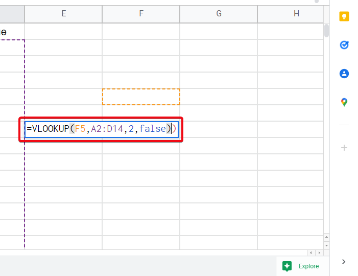
=VLOOKUP(search_key, range, index, [is_sorted])
As you can see from the above VLOOKUP formula:
Let’s break it down
SO, the formula has four variables:
- Search key
- range
- index
- is sorted
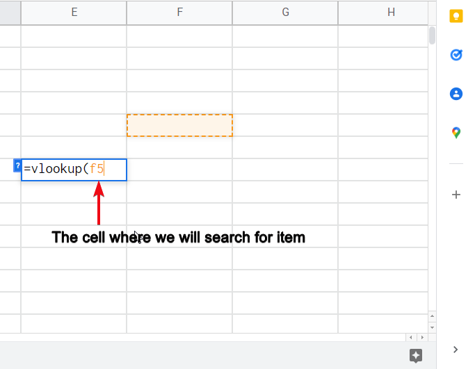
1.Search-Key
is the search term we are looking to search by the VLOOKUP formula, it’s indicated as a cell number where we will write the search item?
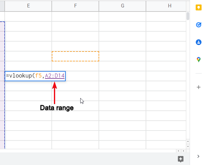
2.Range
The range is the cell ranges of your data that should cover by the VLOOKUP formula.
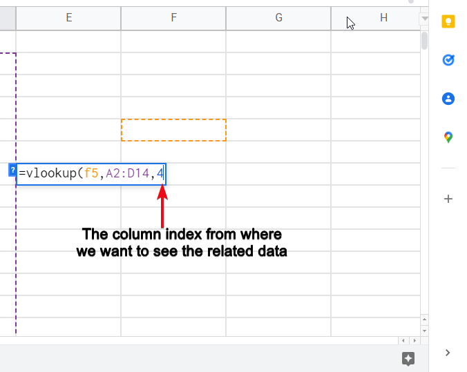
3.Index
The index is the column number from which the related value of the search term should be collected.
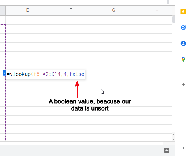
4.Is sorted
It is a Boolean type, it should be true or false, in 99% of cases it is false.
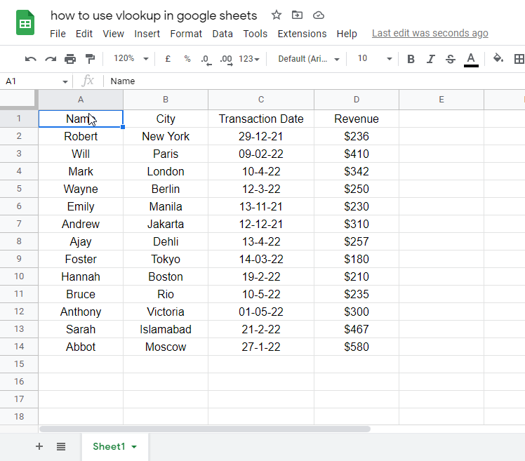
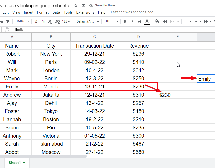
Let’s see an example to implement the above formula
Step 1
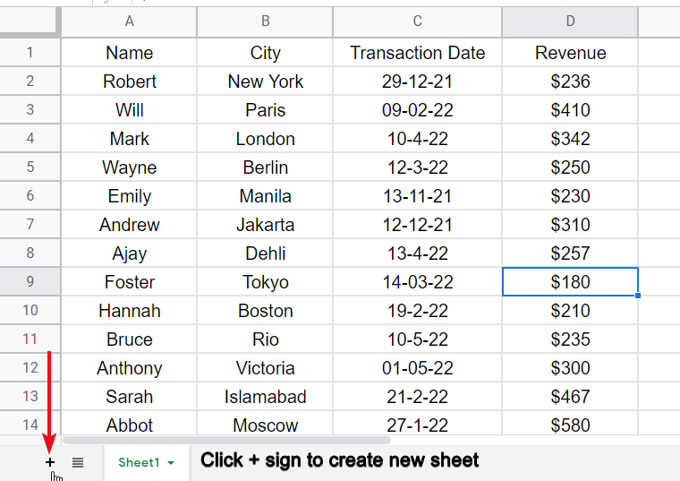
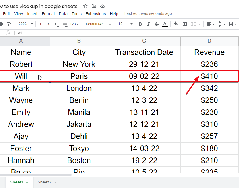
Create some data that have multiple rows and columns
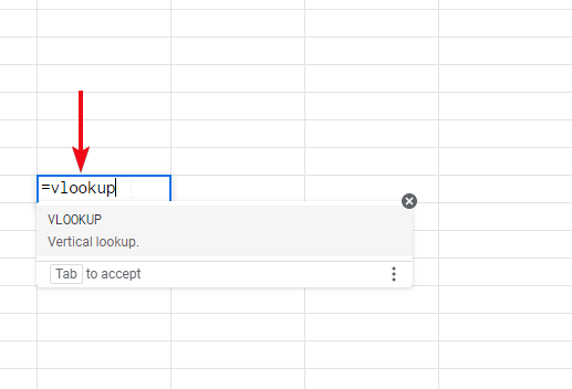
Step 2
in another cell, start writing the VLOOKUP formula
Step 3
Define the first variable
Step 4
Define the second variable
Step 5
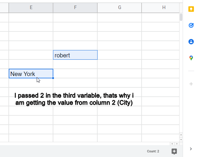
Define the third variable
Step 6
Define the fourth variable
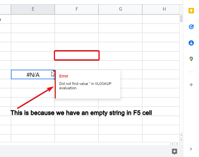
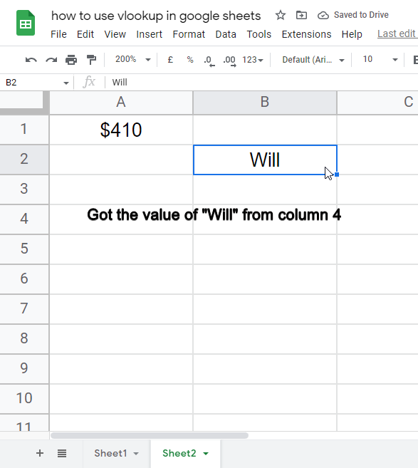
Step 7
Hit Enter, and you will see an error (#N/A), now in the search cell search any name from the list, and the error will be removed, this error is appearing because currently, we have an empty string in the search cell.
Step 8
Testing the VLOOKUP formula.
This is how easily we can use VLOOKUP and search for related items very easily and accurately
How to use the VLOOKUP Function in Google Sheets
The same features can be used using the VLOOKUP formula, in case you like to use the function you can use the VLOOKUP function and pass the values to have the same functionalities.
Let’s see how it works using the built-in function
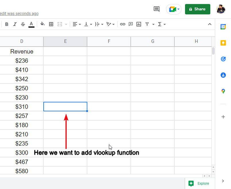
Step 1
Select the cell where you want to keep your VLOOKUP function
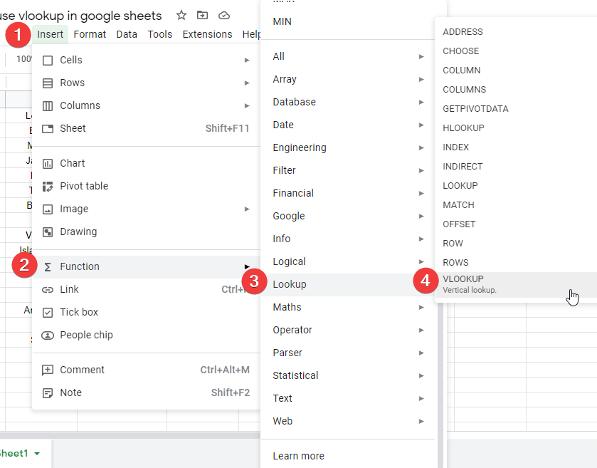
Step 2
Go to Insert > Function > Lookup > VLOOKUP
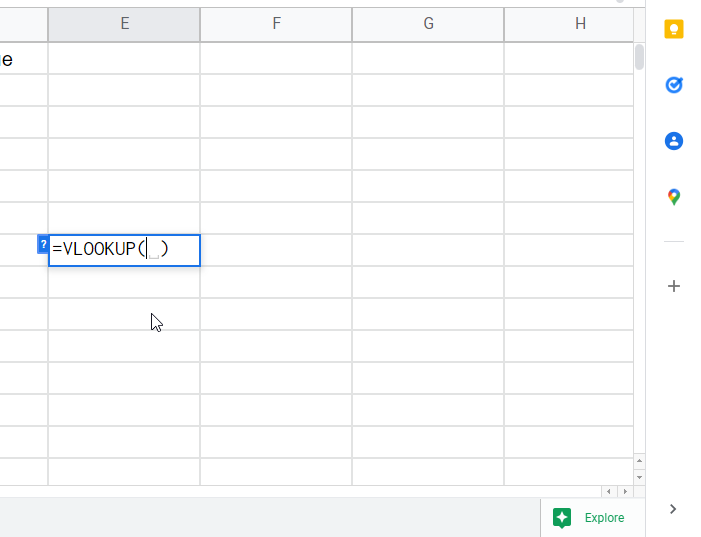
Step 3
The function is ready, now pass the four values.
Step 4
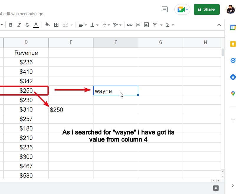
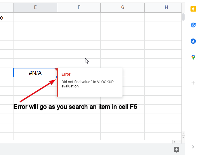
Hit enter and you will see an error message “#N/A”. Error will go as you search an item in cell F5.
Step 5
Search for any item from column 1, and this is how it works.
This is how you can use the VLOOKUP function alternatively to its formula, both are identical and give the same performance and result. It’s just a matter of preference.
How to use VLOOKUP in Multiple Google Sheets
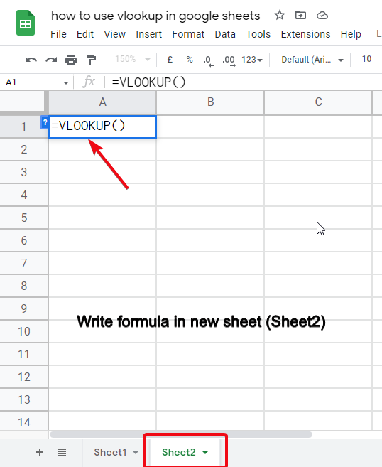
So, in this section, we will explain how to use VLOOKUP in multiple google sheets, note that both the formula method and function method works almost similarly when using multiple sheets in google sheets. We will use the previous example of data and we will how we fetch the same data but on the sheet. Let’s see how it works.
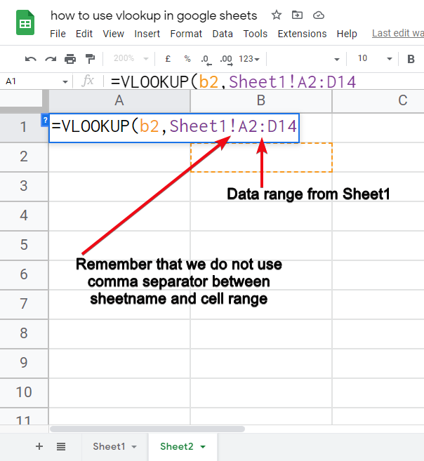
Step 1
As you already have the previous data, simply create a new worksheet
Step 2
In the new worksheet, start writing the formula
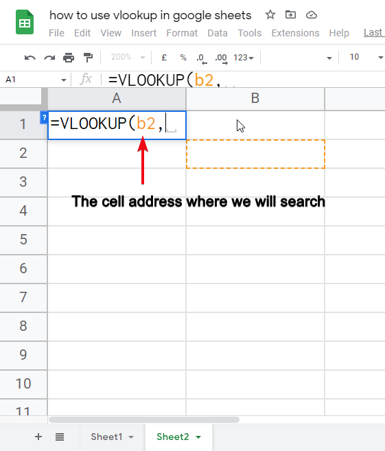
=Vlookup(Search_key,Sheetname!cell_range,Column_index,is_sorted)
- Search key: this is the cell address where we will search for the items
- Sheet name: The sheet name from where we will fetch the data
- Cell-range: The cell range of the entire data on which we are using VLOOKUP
- Column index: The column index from which we want to get the related value
- Is sorted: False when data is not sorted (we use false for 99% of cases)
Step 3
Define the first variable
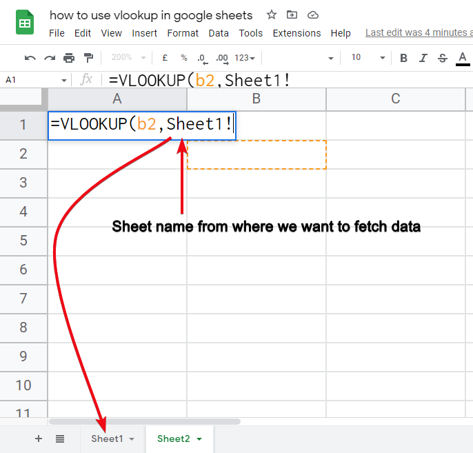
Step 4
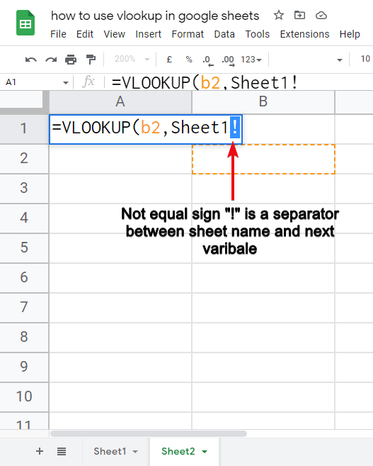
Define the second variable, google sheet ID. Here it is “Sheet1“.
Now put not equal sign “!” after the google sheet ID.
Step 5
Define the third variable
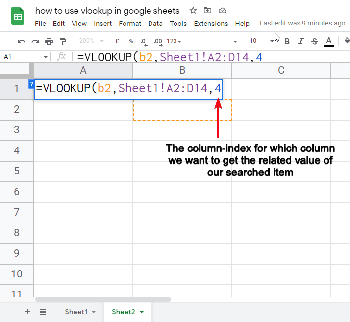
Step 6
Define the fourth variable
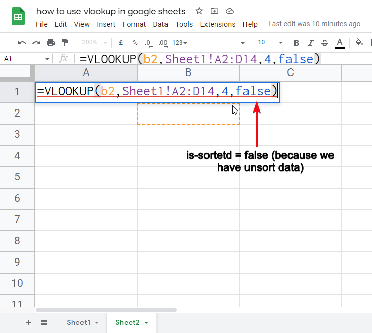
Step 7
Define the fifth variable
Step 8
Hit Enter, (you will see an error that will go when you search something)
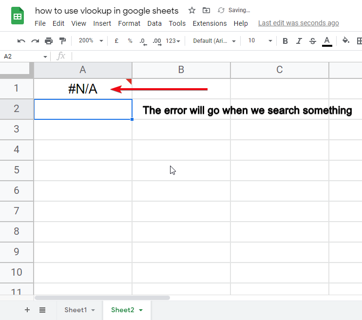
Step 9
Try searching for an item, and you will get the result
This is how easily we get to use VLOOKUP functionalities across multiple sheets, this method is also applicable even when we have hundreds of sheets.
How to use If Error VLOOKUP in Google Sheets
So now, it’s the time to handle some errors, as we have seen VLOOKUP in previous sections, you think of error handling. Look, errors are the part of working with formulas and functions in google sheets, we can’t prevent it but we program what to return when an error appears. So, in this section, we will learn how to if error VLOOKUP in google sheets.
So, we are going to use the same example but this time we will search a term that is not in the list so you can see the VLOOKUP will return an error, then we will apply if error function and again do the same process and you will see how helpful if error function is when working with VLOOKUP.
Step 1
Searching for an item that does not exist
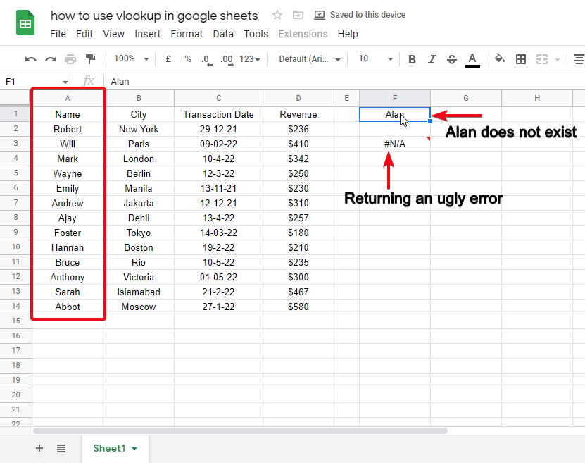
Step 2
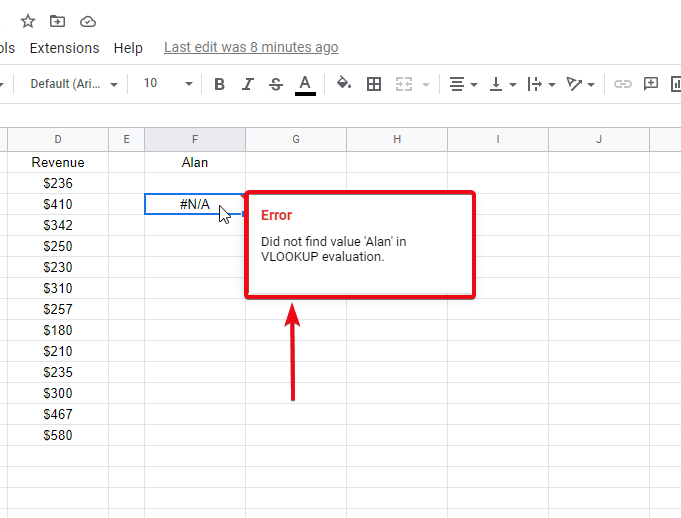
Seeing an error
Step 3
Applying if error to our VLOOKUP formula
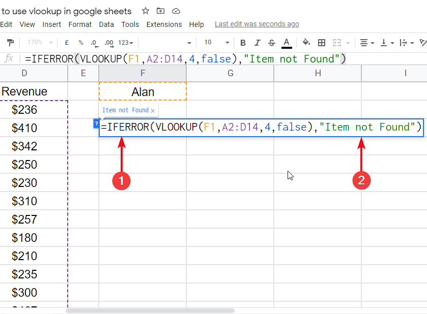
=VLOOKUP(F1,A2:D14,4,false)
=IFERROR(VLOOKUP(F1,A2:D14,4,false),”Your message”)
We will enclose our VLOOKUP formula into IFERROR and after the variables of the VLOOKUP formula, we will, a custom message in double-quotes after a comma.
Step 4
Now, we are getting a meaningful message when an error appears.
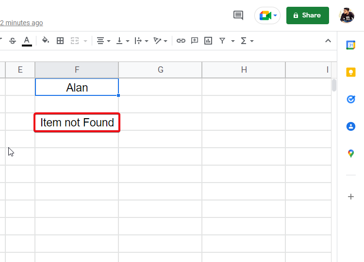
I hope the above use case was helpful to you, you saw how we can handle errors and return some meaningful messages in case of an error.
How to use VLOOKUP and Import Range in Google Sheets
Finally, we are here, the most important and most outstanding feature of VLOOKUP is here, in this section, we will how to use VLOOKUP and import range in google sheets, now keep in mind that VLOOKUP and import range are two different functions, we will use them together in this section we will learn how to use them to bring a searchable data from another sheet. Let’s see how it’s done in the step-by-step procedure below.
Step 1
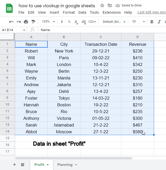
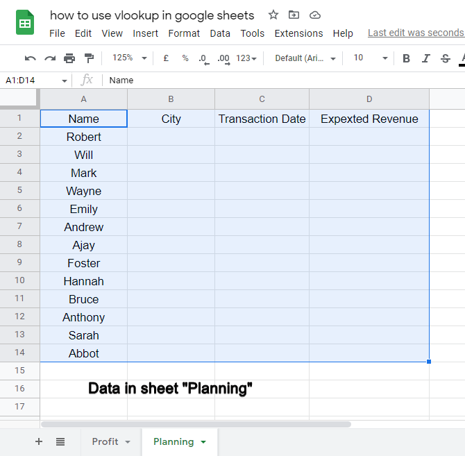
Create two sheets one should have some sample data and the other should have less data
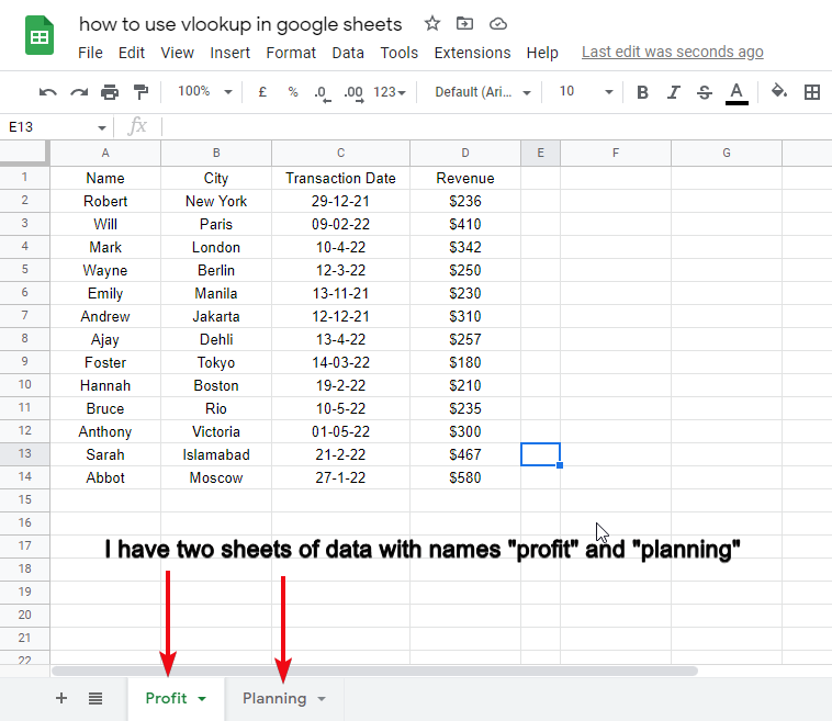
Step 2
we will bring the data into sheet “Planning” from sheet “Profit”
Step 3
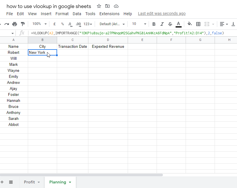
Now in Sheet2, start writing the formula
=VLOOKUP(A2,IMPORTRANGE(“URL”,”Sheet1!A1:F”),3,FALSE)
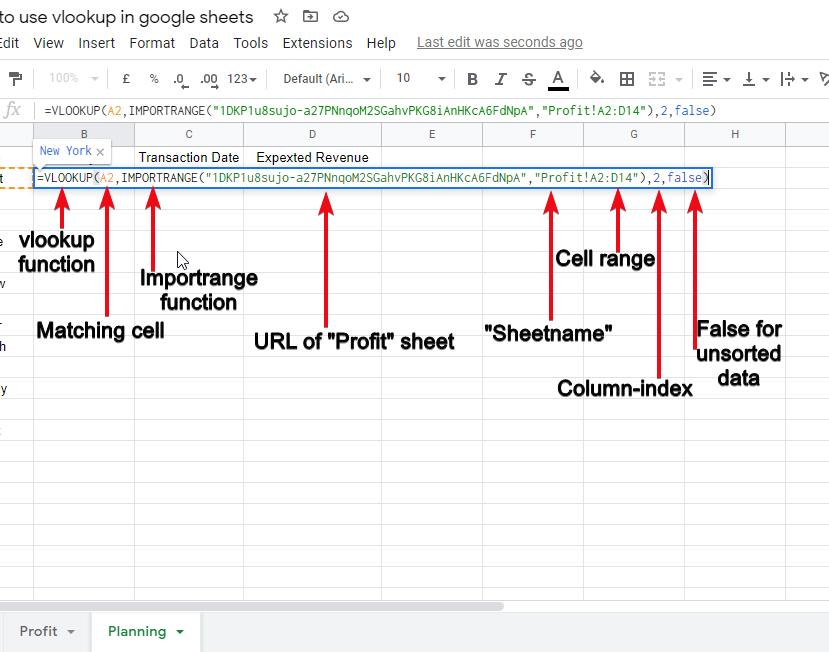
Let’s break down the formula
- A2: is the cell where we will search for the item(s)
- Import range: is another function we are using with VLOOKUP
- URL: is the URL of the sheet1 from which we want to import the data
- Sheet1: is the sheet name from where we are importing the range
- ! Symbol : is the separator between sheet name and date range
- A1:F: is the data range
- 6: is the column-index
- False: is for unsorted data
Step 4
Defining Formula variables
Step 5
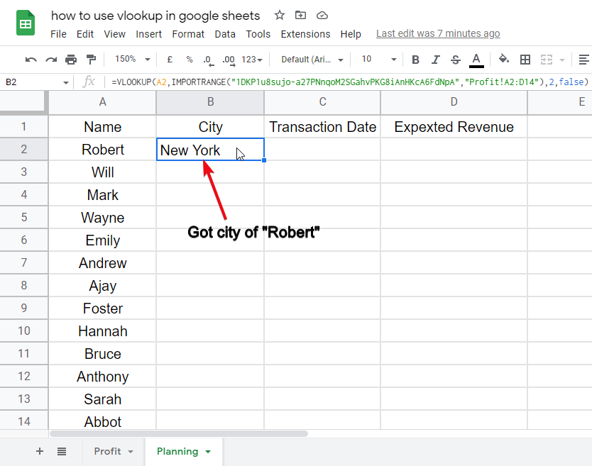
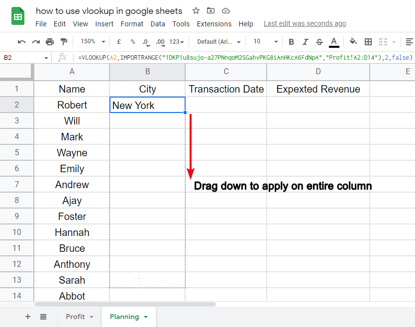
Hit enter and you’re done. We go the city name of Robert as return
Drag down to apply on entire column.
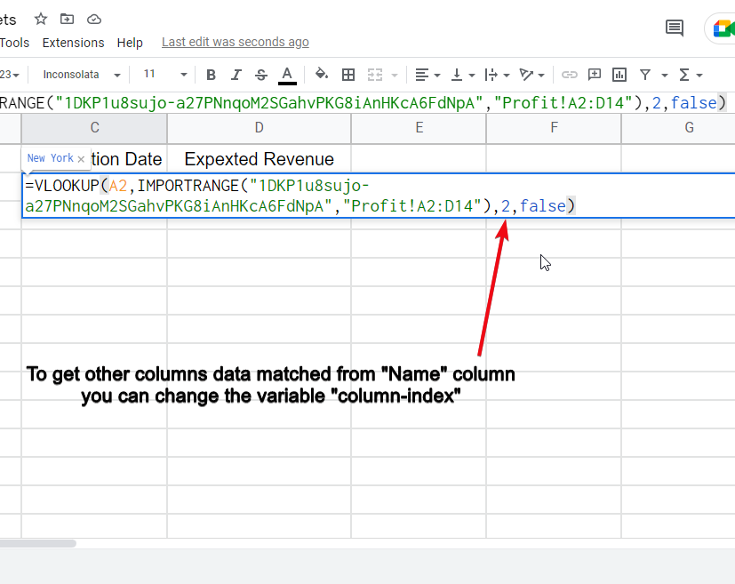
To get other columns data matched from “Name” column you can change the variable “column-index“.
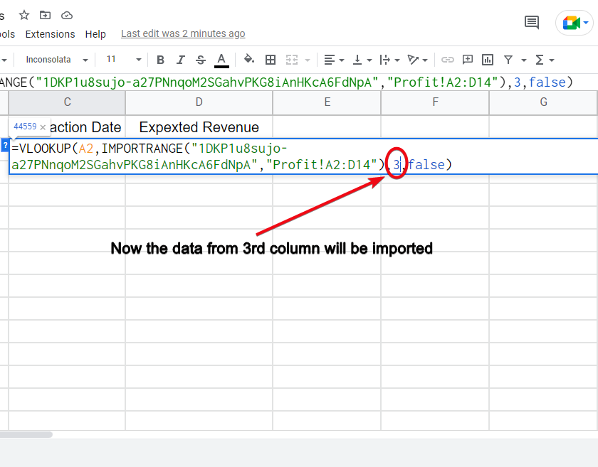
Now the data from 3rd column will be imported.
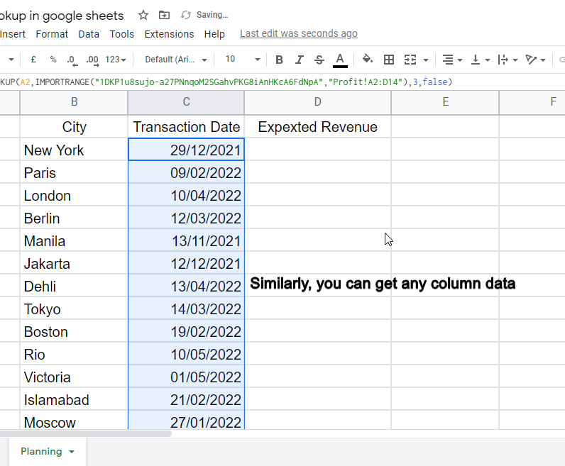
This is how you can combine the import range function with VLOOKUP to import ranges from other sheets.
How to use VLOOKUP for the Interest Rate in Google Sheets
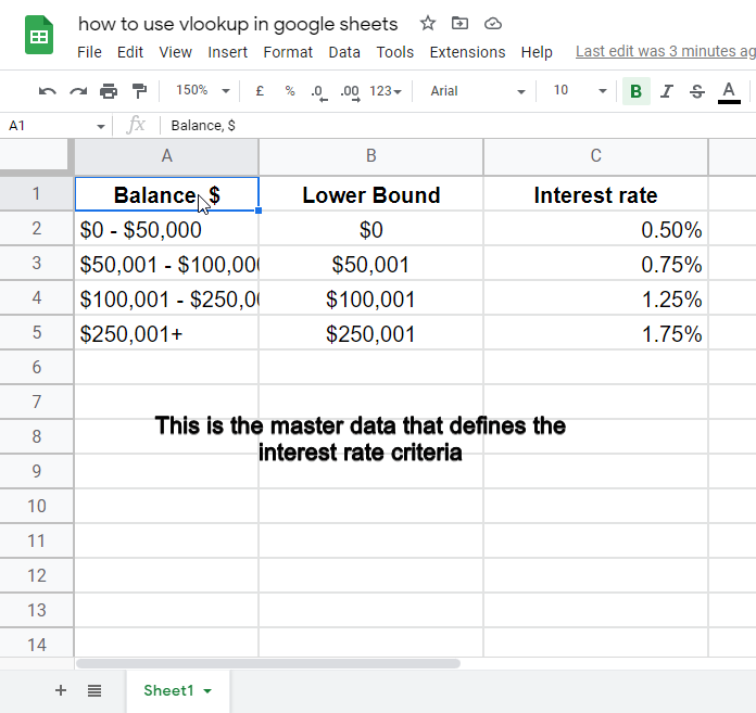
So, in this section, we will see some financial modeling and see how interest rates are calculated using VLOOKUP. In this section, we are going to learn how to use VLOOKUP for the interest rate in google sheets. Let’s understand the example scenario and move to a step-by-step procedure to learn VLOOKUP for the interest rate in google sheets
In the example file, I have the master data that has the conditions for calculating the interest rates of the bank according to the balance.
According to master data information, we will apply a condition to our VLOOKUP function and the interest rate will be automatically calculated. Let’s see how?
Step 1
Make a sheet that defines the conditions of interest rate calculations
Step 2
On the same sheet, make some random account balance list
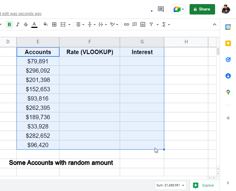
Step 3
Now on the below data, we will use VLOOKUP to calculate the interest rates based on the account balances
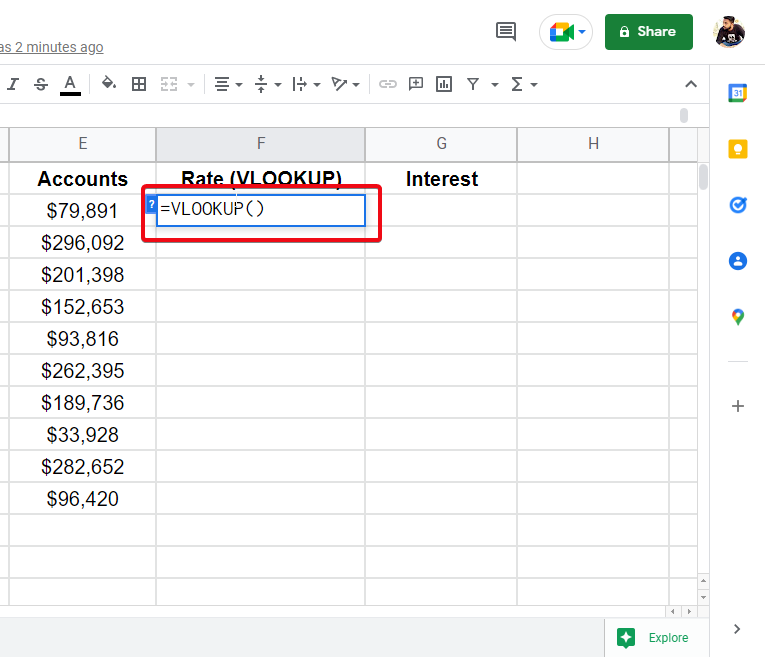
Step 4
The formula
=VLOOKUP(E4,$B$3:$C$7,2, TRUE)
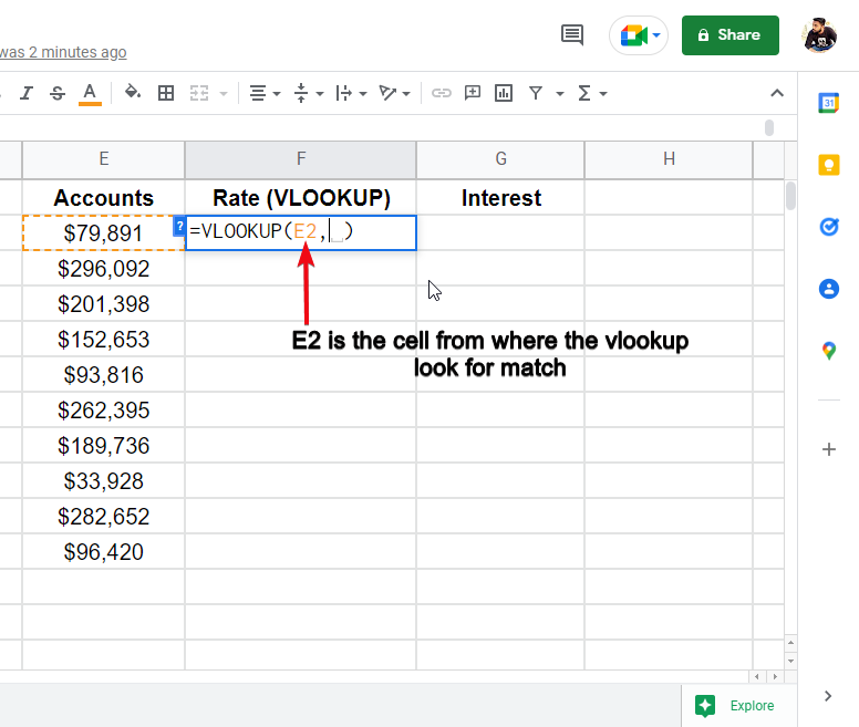
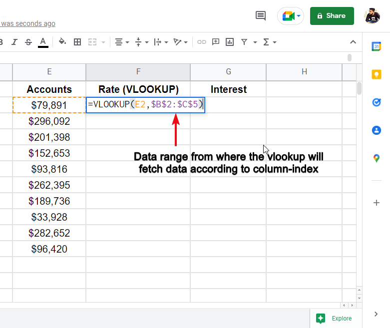
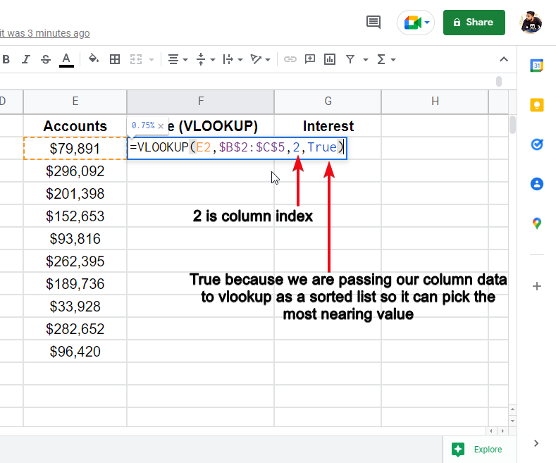
The above formula is quite simple
- E4: The matching cell
- $B$3:$C$7: The cell range from the sheet from where we import
- 2: The column-index
- True: data is not sorted but we want to show it as a sorted data so the function will pick up the least value first
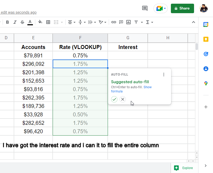
Step 6
Hit Enter and drag for all items
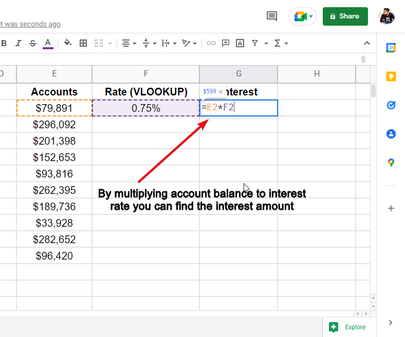
Step 7 (Optional)
Calculate interest amount using simple math operations
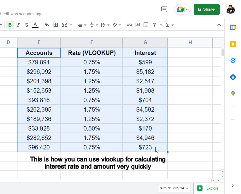
This is how you can use VLOOKUP for the interest rate in google sheets, I hope you find it easy and practice it.
How to use VLOOKUP in Google Sheets for Multiple Returns
Ok, so far so good. We have learned many things regarding VLOOKUP in google sheets, in this section, we are going to see an important feature that is how to use VLOOKUP in google sheets for multiple returns.
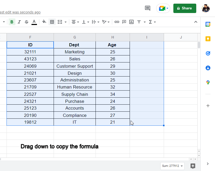
Till now, we were getting one column value from VLOOKUP return, now we will take multiple columns value by writing one single formula and you can return as much columns data as you want:
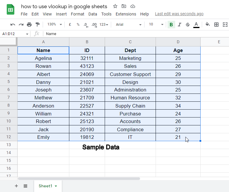
Step 1
Some random data is required to use this function
Step 2
Start writing the formula
=ARRAYFORMULA(VLOOKUP(A2,A2:D12,{2,3,4},FALSE))
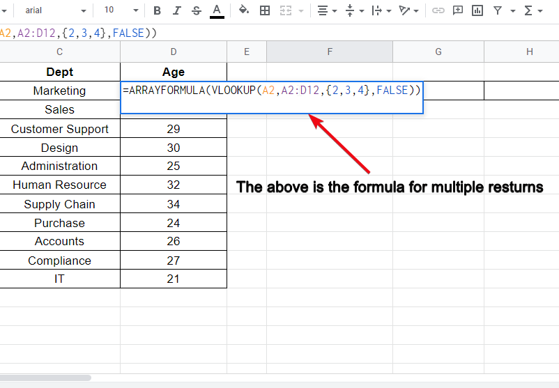
The VLOOKUP formula will be under Array formula syntax.
To return multiple column values we will define our column-index variable inside an array to achieve its functionality.
And the rest formula attributes are defined already many times in previous sections, so I hope you will see that.
Step 3
Hit Enter to execute the formula.
and this way you can use VLOOKUP in google sheets for multiple returns.
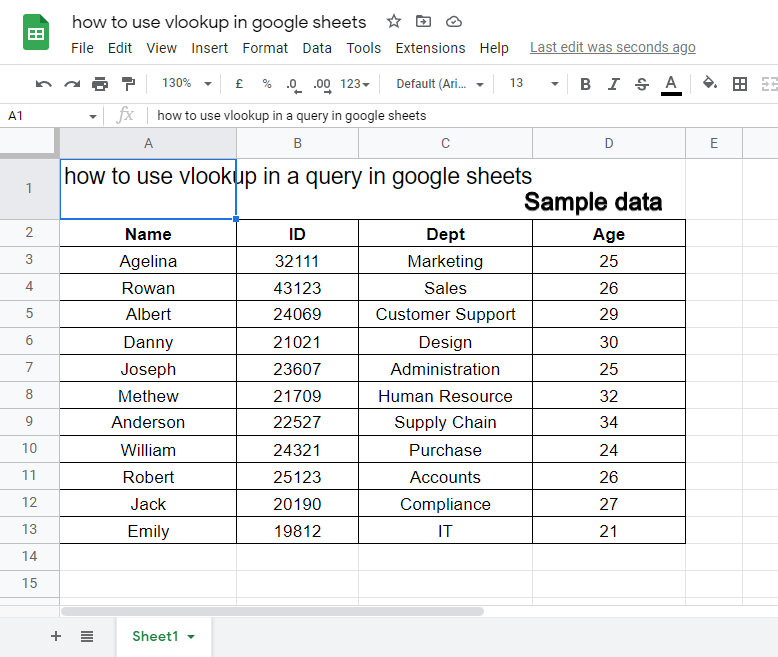
How to use VLOOKUP in a Query in Google Sheets
As we already have learned a lot about VLOOKUP in google sheets, today’s ending section will be regarding VLOOKUP in query, so we will see how to use VLOOKUP in a query in google sheets. We will try to identify the problem statement and an example to learn the solution very easily.
Let’s proceed to the steps required to use VLOOKUP in a query in google sheets.
Step 1
We need a sample data
Step 2
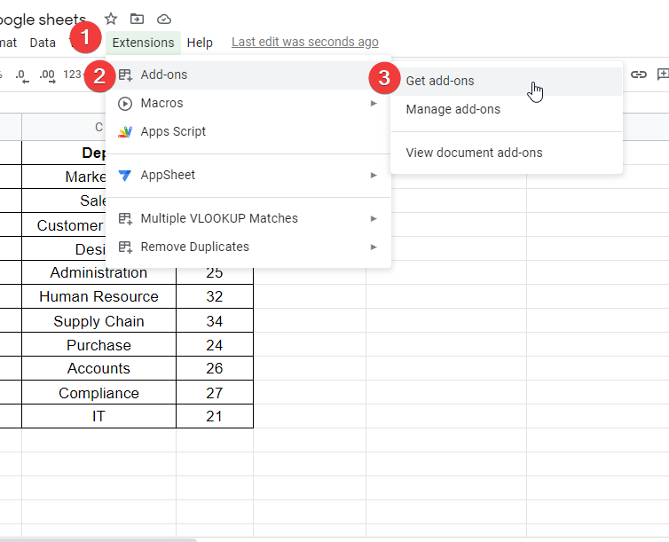
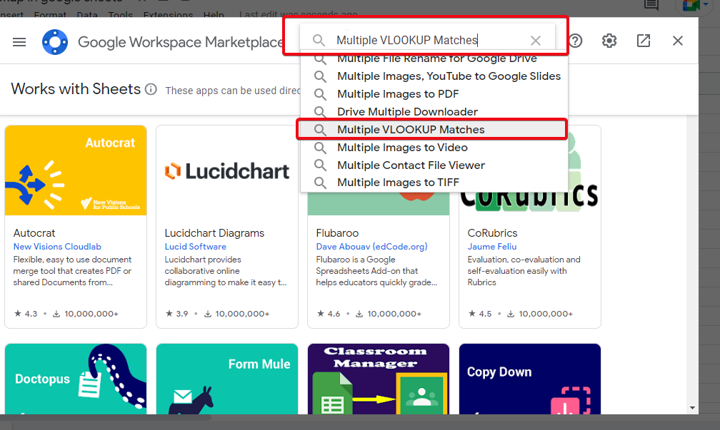
We need “Multiple VLOOKUP Matches” add-on
for this go to Extension > add-ons > get add-ons
Step 3
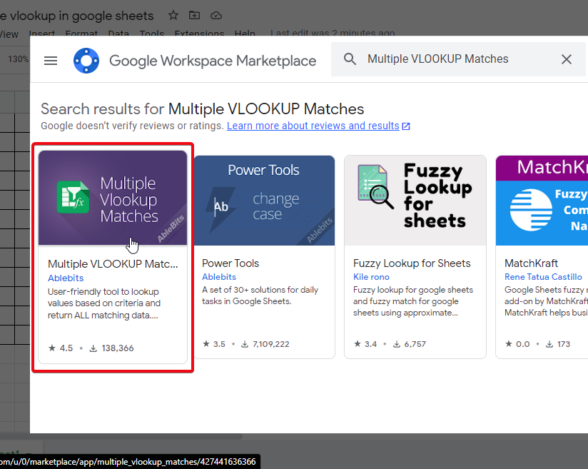
Search for “Multiple VLOOKUP Matches”
Step 4
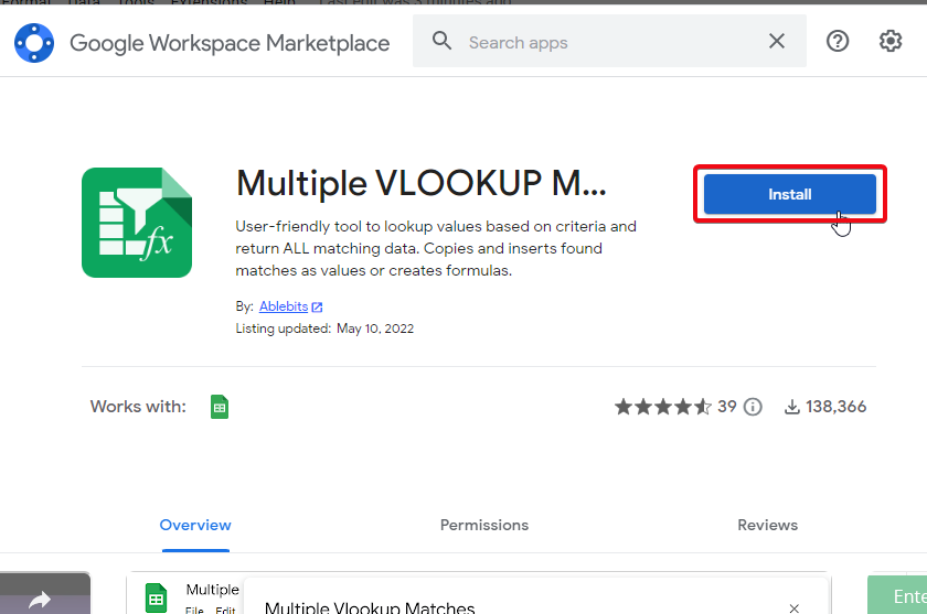
Install “Multiple VLOOKUP Matches”
Step 5
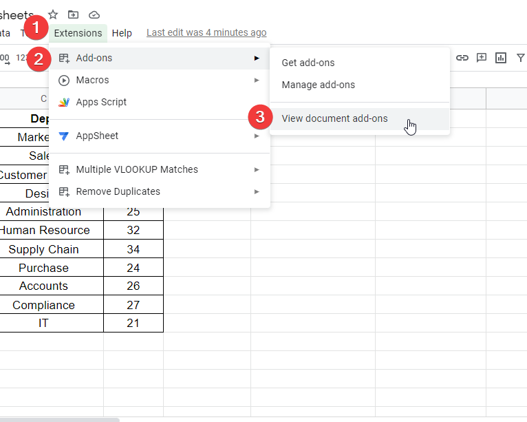
Go to Extension > add-ons > view document add-ons
Step 6
In the add-on window, click use > start
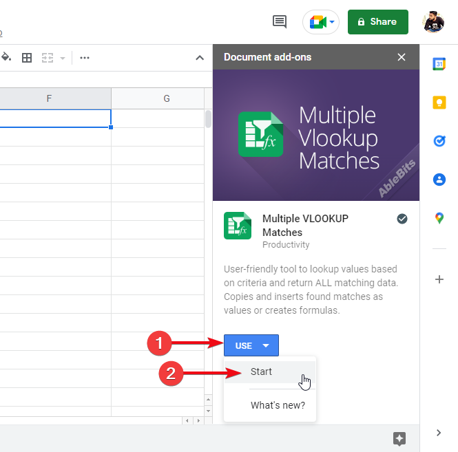
Step 7
Specifying the conditions to generate a query
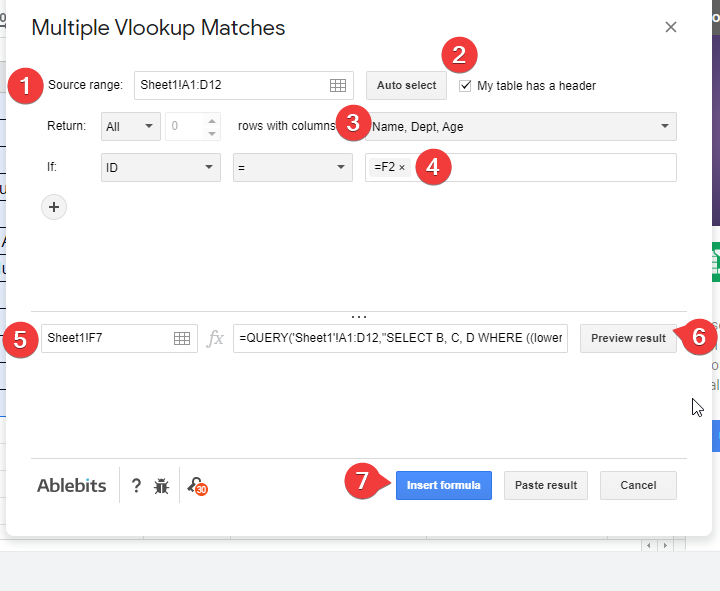
Step 8
Back to the sheet and perform some testing
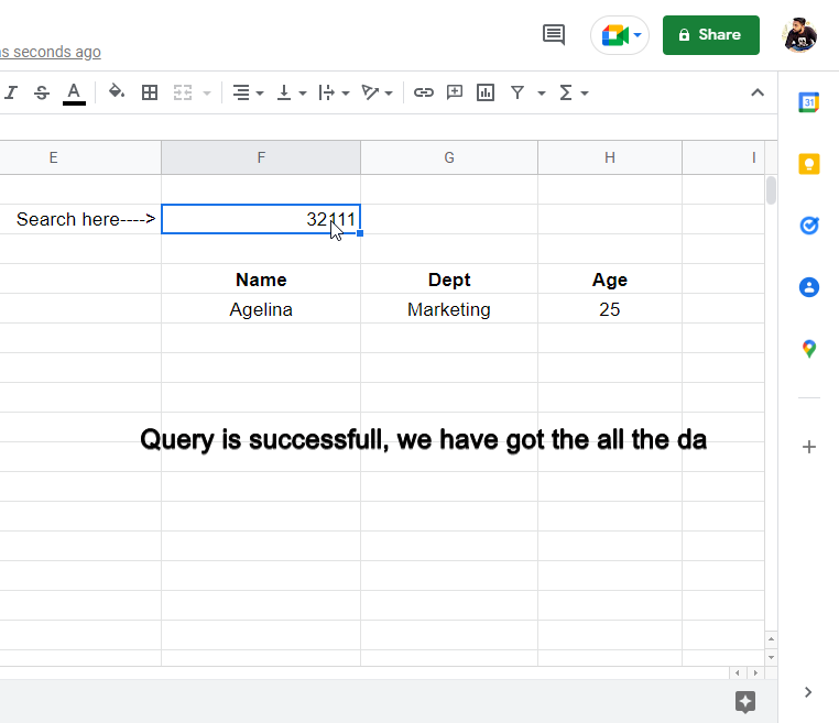
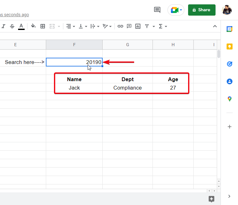
So, this is how easily you can generate a query for using VLOOKUP in google sheets and fetch multiple columns easily/
I hope you found it easy, it was a bit lengthy but it’s not difficult, the add-on is highly interactive and user-friendly.
Some Important Notes about VLOOKUP Formula
- Always remember, that the VLOOKUP formula or function returns a single value until you add the array function.
- When working on multiple sheets, always remember that anything in double quotes always is written in single quotes if required to separate.
- In the “sheet name” variable of multiple sheets VLOOKUP we separate the sheet name from cell range using a ! not equal to or inverted exclamation mark replaced with a comma.
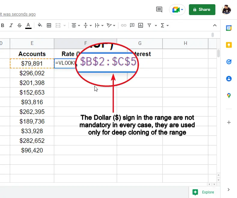
- $ Dollar sign in cell range is nothing but for deep cloning only
- When working with multiple sheets, the lookup formula required the URL of the sheet where to import data, the URL required for this function is between /d/ —- /edit. (/d/ URL /edit)
Conclusion
So, how was today’s article? I hope you guys love it, and in this article, we have learned VLOOKUP in very detail and solved 7 problem statements with the help of query, functions, array formula, if error, multiple returns, multiple sheets, and much more. I hope you have learned all the topics covered in this article. If you like our articles please share them with your friends and subscribe to the OfficeDemy blog for exciting updates.


