How to use ISNUMBER in Google Sheets [Guide 2023]

In this article, will learn how to use ISNUMBER function in Google Sheets. ISNUMBER function is simply a function that tells you whether the specified cell address has a numeric value or a non-numeric value. It is used to check between a Boolean value and it only returns TRUE or FALSE.

But this is not enough, this function is primarily used with other functions to make a combination and get useful results such as it is widely used with IF function, and conditional formatting rules, to perform a specific task or print a specific message, and apply some conditional formatting based on the result of ISNUMBER function. In this article, we will learn the common uses of ISNUMBER function with step-by-step procedures and simple examples.

Use Case of ISNUMBER Function in Google Sheets

We often perform calculations on large data sets and get a final result in a cell, but have you ever thought if any of the values in such a large data set is a non-numeric value, then the overall calculator may hurt? Right, so to validate that the value is actually a number in the eyes of google sheets, we have the ISNUMBER function as the top favorite to check if its a number of any other data type, but you can think that number will be written as the number and it can be seen at a glance without any formula or function to check it.

If I write a number apply formatting on it with center align and convert its format into String, then no one on the planet is going to identify it at a glance, you just need to have some tricks some steps to check either its a number or a String or text or anything, so ISNUMBER makes it absolutely simple to validate a data type. A similar concept is used in JavaScript that used a typeof operator to check the data type, and some of you who have done JavaScript must understand the importance of this concept. So, therefore, we need to learn how to use ISNUMBER function in google sheets.

How to use ISNUMBER in Google Sheets

Here we will see how ISNUMBER helps us in many ways, we will learn the step-by-step procedure to master the ISNUMBE function in google sheets. So let’s get started with the basic syntax of this function and then move forward with examples.

ISNUMBER in Google Sheets – Syntax

=ISNUMBER(value)

Here,

value: It can be a value, and most probably a cell address to validate whether it’s a number or other data type.

Tip: ISNUMBER returns TRUE if the value is a number and FALSE otherwise.

This function is frequently used with the combination of the IF function in conditional statements.

Note that passing a number enclosed in double or single quotes  (e.g. ISNUMBER(“421”), or ISNUMBER(‘313’)) will return FALSE because the number passed inside double or single quotes are strings and not numbers.

ISNUMBER Function in Google Sheets – Simple Usage

In this section, we will learn how to use ISNUMBER function in google sheets as a very simple usage, we will use ISNUMBER solely to see how it works and how it validates data types.

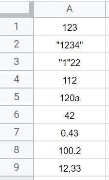
For this example, I have some sample data written in column A, and I will apply ISNUMBER in column B and I will get the TRUE or FASLE values corresponding to the values written in column A

Step 1

Sample data

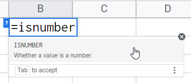
Step 2

Type the ISNUMBER function

Step 3

Pass the cell address (A1)

Step 4

Press Enter key, and you get the result

Step 5

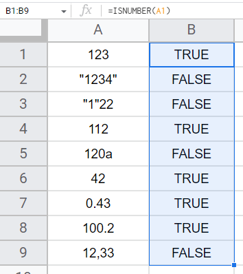
Copy the formula below to apply the formula to the entire column A

Step 6

Explanation of results

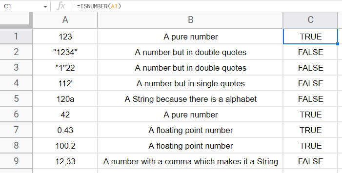
This is how you can see the ISNUMBER function returned TRUE for numbers and false otherwise.

But it does not seem to be a useful use case of the ISNUMBER function, it does not make sense. Now, we will see some useful applications of ISNUMBER combined with other functions.

ISNUMBER Function in Google Sheets – with IF Function

In this section, we will learn how to use ISNUMBER function in google sheets with the IF function. We will validate if the value is actually a number and if TRUE we will perform some calculation, and if not then we will print a custom message. This way we can avoid having ugly reference errors, and type errors.

For this example I have a data set in which I have some numbers and a few strings, strings are disguised like numbers, so we will find them out using our custom formula made up of the combination of IF and ISNUMBER functions

Step 1

Sample data

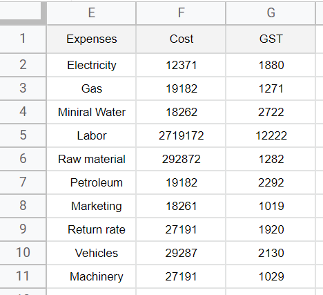
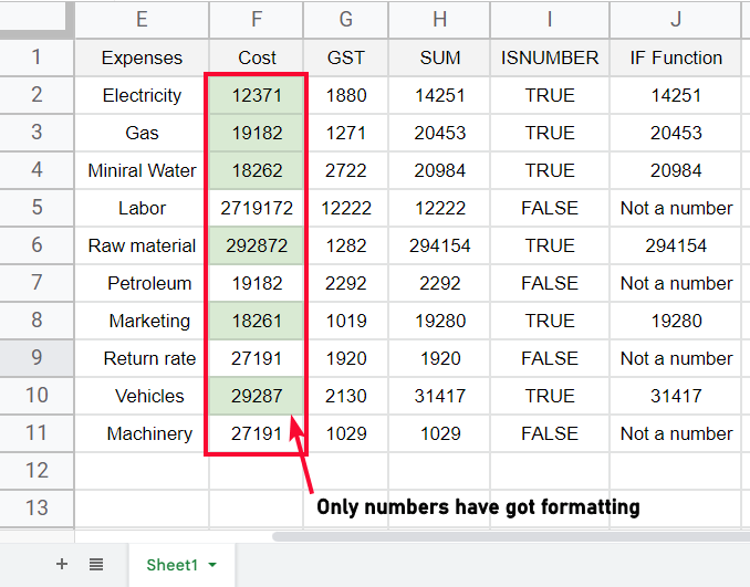
Tip: You can see all values are looking like numbers in the Cost column, but there are some text and String values that can not be detected at a glance

Step 2

Tip: We need to calculate the total cost and GST for each expense.

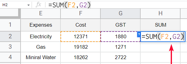
Apply a simple sum formula for Cost and GST

Step 3

Here is the result, but wait have you noticed, that some values are not summed up and they are showing only the two values

Step 4

Apply the ISNUMBER function and check each value in the cost column

Step 5

Now you can see some of them are not numbers and that’s why they did not sum up

Tip: Now we need to use the IF function with ISNUMBER and SUM

Step 6

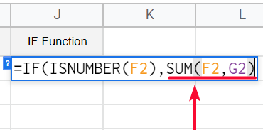
Type the IF function

Step 7

Pass the ISNUMBER as the first argument of the IF function

Step 8

Pass the cell reference (to validate) inside the ISNUMBER function

Step 9

Now pass the SUM function with the cell reference of Cost and GST columns to be summed if the condition (in the ISNUMBER function) is true

Step 10

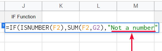
Now specify a custom message (inside double quotes) to print if the condition is FALSE

Step 11

This is what you get using the IF function with ISNUMBER

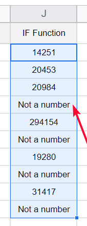
The values which are actually numbers are summed by function, and the values which are not numbers are detected and the IF function through them into the else block, and thus we avoided getting the wrong value in the calculation of SUM of 1 number, and 1 String.

I hope you find this very helpful, and trust me it’s a real-world use case of ISNUMBER and IF Function, you can see how helpful it is.

Let’s move on and learn another helpful use case of the ISNUMBER function along with conditional formatting rules.

ISNUMBER Function in Google Sheets – with Conditional Formatting

In this section, we will learn how to use ISNUMBER function in google sheets with conditional formatting, we will learn how to combine this with conditional formatting rules and apply formatting to the content based on its data type.

So, let’s further simplify the previous problem, the previous problem told us that some values are actually strings, so to detect them, we can apply conditional formatting on the values which are considered as non-numeric values by the ISNUMBER function, so that we can change them.

Step 1

Same data set

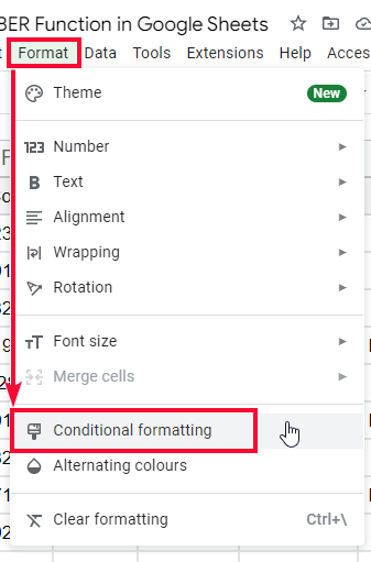
Step 2

Go to Format > Conditional formatting

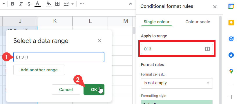
Step 3

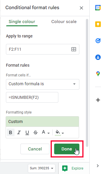
Select your entire data range in the Apply to range section

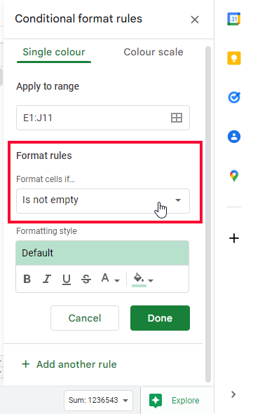
Step 4

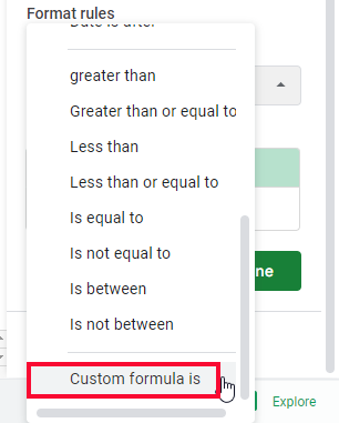
From the below Format rules section select a condition to apply the formatting, here select “custom formula is”

Step 5

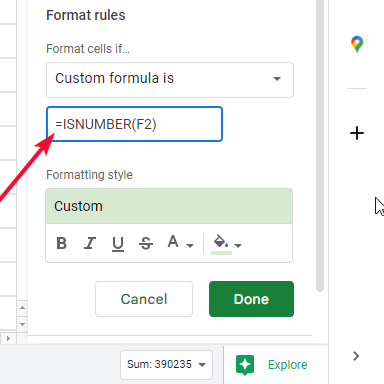
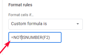
Now you need to pass a value of the formula; here we will pass the ISNUMBER function

=ISNUMBER(F2)

Step 6

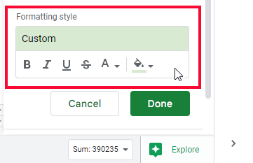
From the below formatting style section, select some formatting; cell color, text color, bold, underline, italic, etc. You can use any of the formatting styles or multiples to be applied to the cells that satisfy the above condition

Step 7

Click on done.

Step 8

Now you can see all the values which are numbers have got the formatting, now you can detect the values which are looking like numbers, but are not numbers in reality.

Probably you find your data a bit messy by having too many colors in the cells having numbers, you can reverse the logic and only apply formatting to cells that are not numbers from specific columns, to do this follow the below steps

You only need to reverse this function, if you remember we have already covered NOT function in this series of articles.

Step 1

Type NOT function at the starting of the ISNUMBER function

Step 2

Add brackets of NOT function

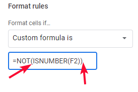
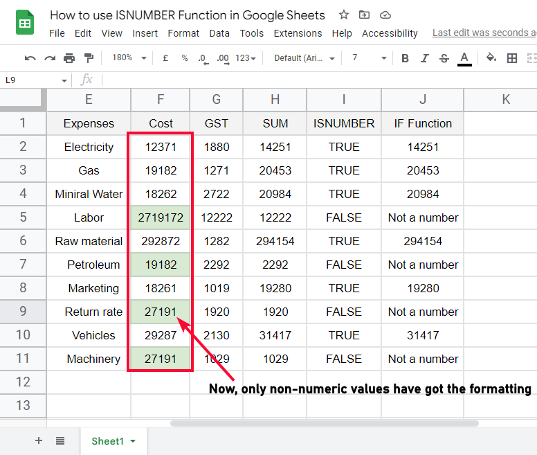
Step 3

Now you can see the logic is reversed and now only non-numeric values are formatted, you can also change the color to red to know that they are the error values.

So, these were the real-world applications of ISNUMBER functions with other functions like IF and concepts like conditional formatting, and also the NOT function. I hope you have learned the usage and importance of the ISNUMBER function in google sheets.

Download/Copy Google Sheets Workbook

Important Notes

Conclusion

Wrapping up how to use ISNUMBER function in google sheets, we learned the syntax first which was very easy then saw a simple usage of the function and after that, we learned two of the most important and most used use cases of ISNUMBER function, one along with IF function and the second with conditional formatting.

I hope you find this tutorial helpful and that now you have learned how to use ISNUMBER function in google sheets. I will see you soon with another helpful article, till then take care. Keep learning with Office Demy.