How to Link Google Sheets Together [3 Methods]

In this guide, I will teach you how to link Google Sheets together. Spreadsheet software is the best way to organize data on different Sheets. Similarly, linking data from multiple spreadsheets can be fantastic for analyzing exact data across a range of cells in different Sheets.

Today’s topic is how to link Google Sheets, so let’s start.

Why do we need to Link Google Sheets Together?

If your data is on different Sheets and you want to gather it on one sheet for some calculations, then you don’t need to write down all the data again, but you can import them or create a link between them.

Therefore, you may need to link Google Sheets together which we are going to learn in the following article on how to link Google Sheets together.

How to Link Google Sheets Together?

Google Sheets links Sheets together in many cases, In the following tutorial on how to link Google Sheets together, we will learn some of them that are below.

1. Link Google Sheets together by inserting a link
2. Link Google Sheets together by applying the formula
3. Link Google Sheets together by Importrange

Link Google Sheets Together – By inserting a link

The most straightforward way of linking Sheets together in Google Sheets is to create a link between Sheets through which you can easily access any sheet anywhere with just one click. Let me show you practically by applying this in the following steps.

Step 1

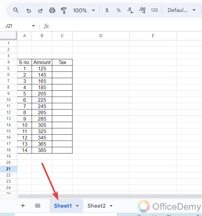
As we are going to link multiple Sheets, here in the following example, you can see we have 2 different Sheets and right now we are on sheet 1 with some tabular data as can be seen below.

Step 2

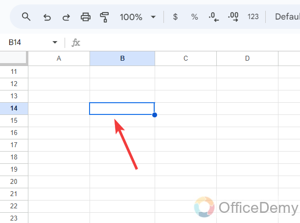
To link one or more Sheets, first, we will navigate to any cell on the sheet we want to link. Here we are on Sheet2 and have selected a cell to ia insert a link with sheeet1.

Step 3

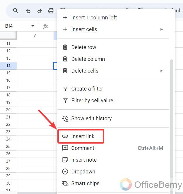
To insert a Link, press the right click of the mouse into the following selected cell, and a drop-down menu will open where you will see an “Insert Link” option as highlighted in the next picture. Click on it to insert a link.

Step 4

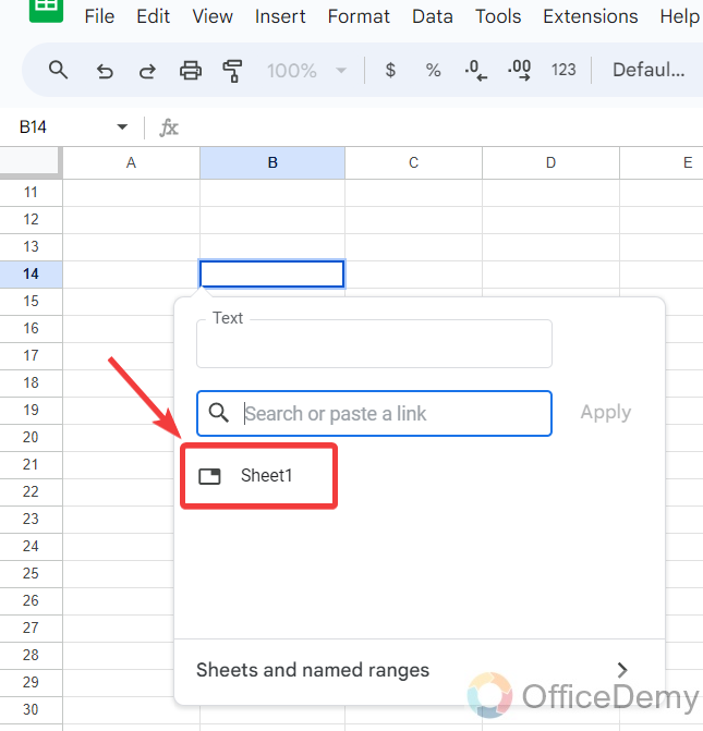
When you click on the “Insert Link” option, the following drop box will appear along the selected cell, on this Dropbox Google Sheets will ask you to insert a link where you can simply write the name of the sheet (e:g Sheet1 or any name) and at the other hand, you can also simply select the sheet from suggestions as I have selected below.

Step 5

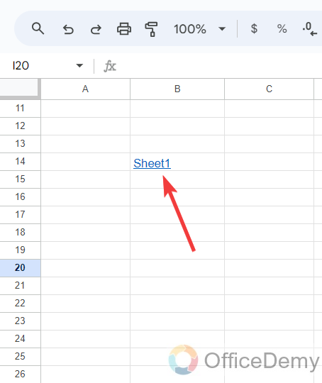
As you select the Sheet that you want to link with the active sheet, the link will be inserted into the cell through which you can easily access the given sheet as you can also see in the following picture, the cell text has turned into blue that’s mean Link has been inserted.

Step 6

Let me show you a transition below, how it works and how can we link Google Sheets with each other.

In this simple way, you can link Google Sheets together.

Link Google Sheets Together – By applying a formula

If you are applying any formula in your Google Sheets, but the required data is on two different Sheets, Google Sheets allows you to insert range from another sheet as well. In this way, Google Sheets creates a link between two separate Sheets. When you change any value on the other sheet it will automatically impact the calculation on the first sheet. Here is an example of this method of linking Sheets together.

Step 1

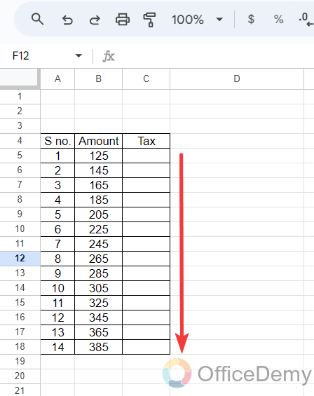
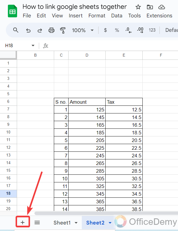
Let’s suppose this is sample data on which you are currently working. As you can see in the following picture, in this sample data we are finding the applicable tax amount on the given amount.

Step 2

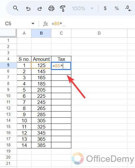
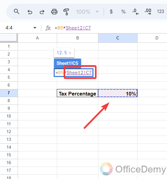
To find the tax amount, we simply apply the multiplication formula, as we know the applicable tax rate which is on the other Sheet. Let’s see how we can link these Sheets by applying the simple formula.

Step 3

While giving the cell range, just navigate to the other sheet and select the cell range, Google Sheets will automatically link the first sheet to the other one. Once you have written a formula then hit the Enter key, Let’s see does it works or not.

Step 4

By pressing the Enter key, the result is in front of you as you can see in the following picture. Although we have taken value from another sheet in the applied formula Google Sheets automatically link the Sheets.

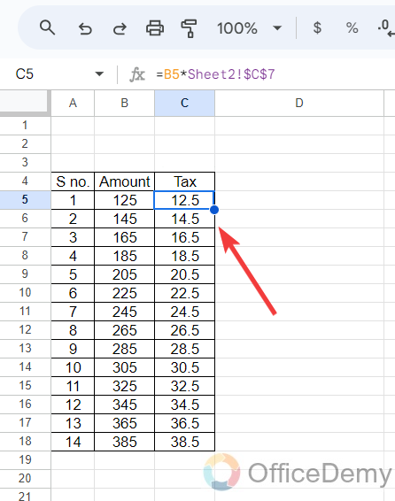
Step 5

This link feature works amazingly, if you change the value on another sheet, Google Sheets will automatically recalculate the expression as you can see in the demo in the following animation.

Link Google Sheets Together – By Importrange Function

Let’s suppose you have a table on one sheet, and you have required the same data on another sheet. Yes, you may simply copy it, but it will not automate the values when you make changes in one sheet. But if you use the Importrange function, it will not only copy your data to another sheet but also automate your sheet whenever you make changes to the source sheet. Google Sheets links Sheets together with the help of the Importrange function to automate data.

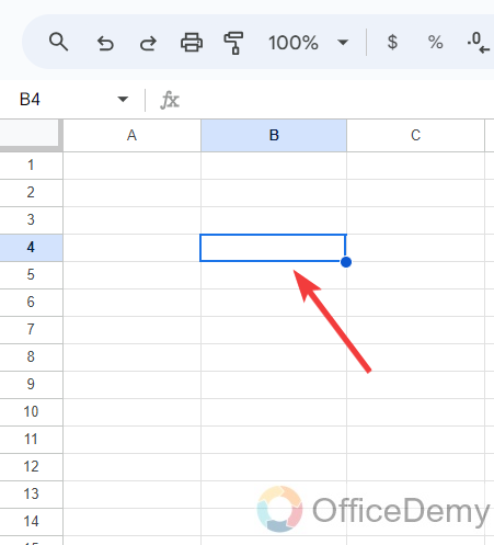
Step 1

After adding a new sheet, first, navigate the cell where you want to apply the “Importrange” formula as I have selected below.

Step 2

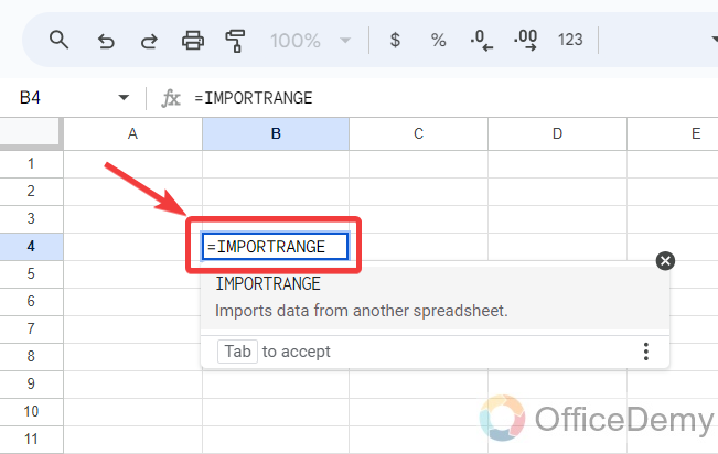
In Google Sheets, every formula starts with an equal sign, so we will write first an “Equal” sign to start the formula then we will write the name of the formula that we want to apply as I have written the “Importrange” formula.

Step 3

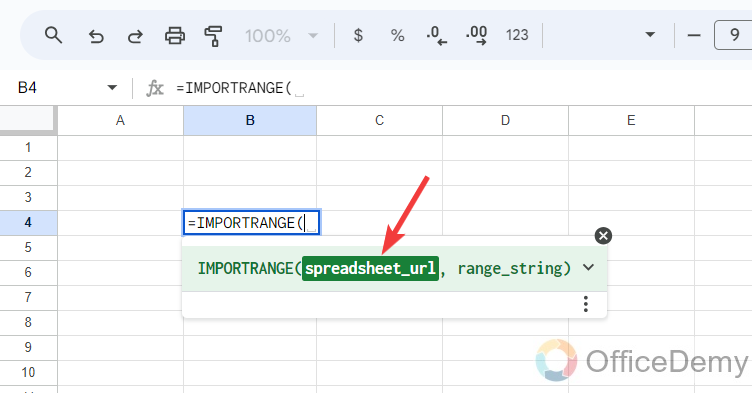
After writing the formula, when you write a small bracket, Google Sheets will automatically suggest other variables to complete the formula, as here you can see the first suggestion, it is asking for “Spreadsheet _URL“.

Step 4

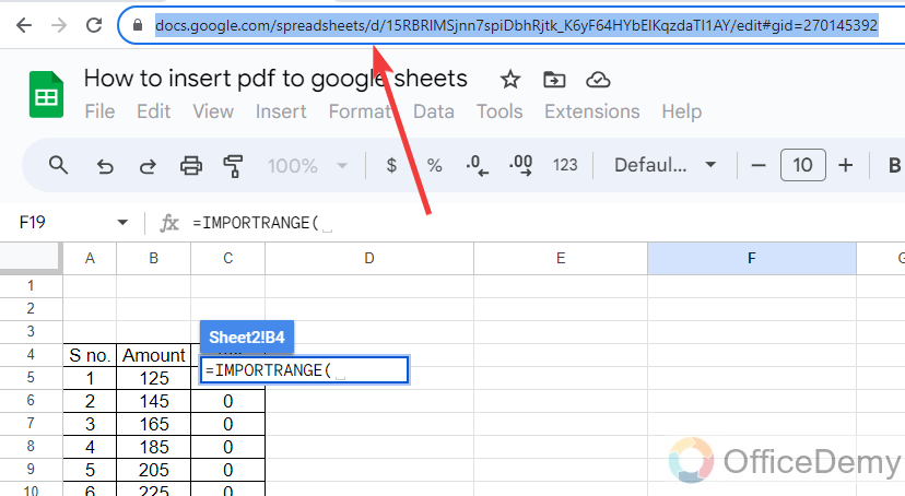
To Insert the sheet URL, come to the sheet from where you are importing data, copy the URL from the URL bar as directed in the following picture, and then paste it into the Importrange formula.

Step 5

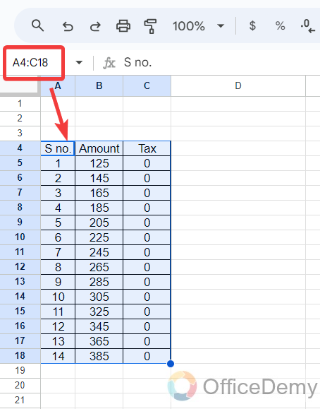
After writing the spreadsheet URL, in the next parameter, you will have to give the data range that you want to import to the other sheet, you can copy the data range from the following cell range box by selecting the data and then putting it into the syntax.

Step 6

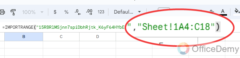
Watch the pattern of writing these parameters in the syntax to prevent any kind of error. Must be careful with all commas, inverted commas, and exclamation marks.

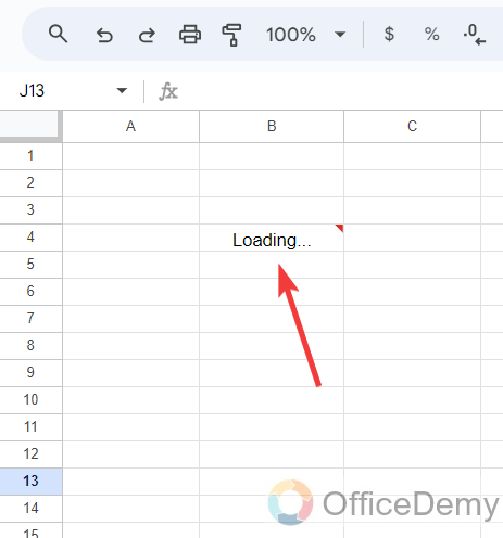
Step 7

Once you are done with writing the formula of importing range, when you press the Enter button to get the result, it will take a few seconds and indicate you are “Loading” as can be seen in the following picture.

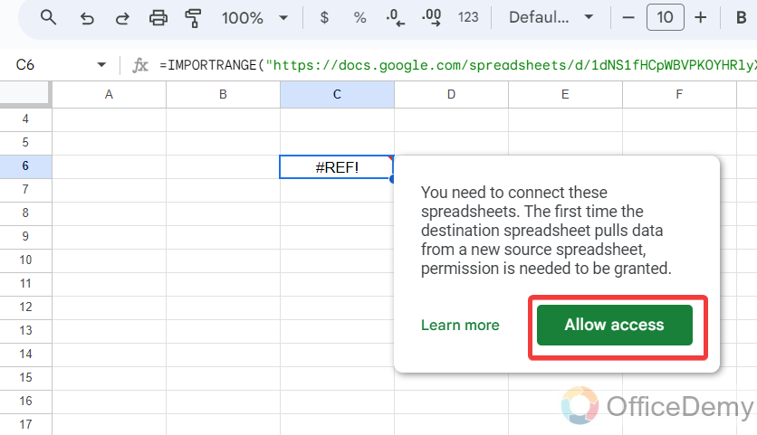
Step 8

After a while of loading data, you will get an error (=REF), but there is nothing to worry about, just hover the cursor over it, and you will get a prompt message that will ask you to grant permission to import data. Click on the “Allow access” button.

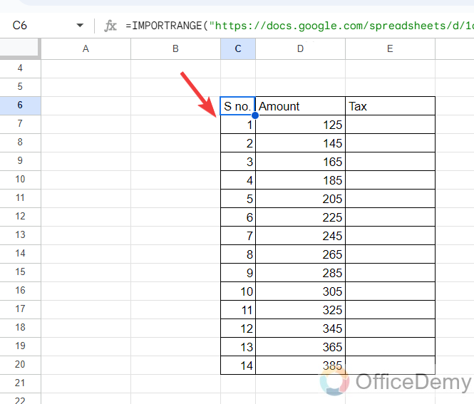
Step 9

As you click on the “Allow access” button, your data will instantly import to the following sheet as can be seen in the following picture.

Step 10

This importrange formula will create an interaction between the Sheets that when you edit the source data from the first sheet, the import data in the second sheet will automatically change as can be seen in the following animation.

Frequently Asked Questions

Are the Methods for Removing Hyperlinks in Google Sheets Similar to Linking Sheets?

Removing hyperlinks in google sheets is a different process compared to linking sheets. While linking sheets allows establishing connections between different sheets, removing hyperlinks in Google Sheets involves a specific procedure to eliminate existing hyperlink values. Although both involve manipulation of links, they serve distinct purposes within the Google Sheets environment.

Q: How to add a sheet in Google Sheets?

A: By default, there are two Sheets in a spreadsheet Google Sheets but if you want to add more you can add more Sheets by just clicking on the add button that you can see in the following guide.

Step 1

If you look at the left bottom of the Google Sheets window, you will see a “Plus” sign as directed in the following picture. Click on it to add a sheet in Google Sheets.

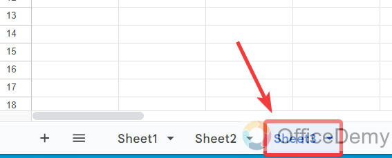
Step 2

As you can see from the result in the following picture, a sheet has been added to the spreadsheet.

Q: How to rename the sheet in Google Sheets?

A: Google Sheets also offers the feature of naming your Sheets, if you want to give a name to your sheet in Google Sheets, below are the steps.

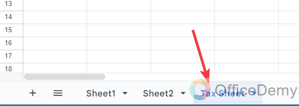
Step 1

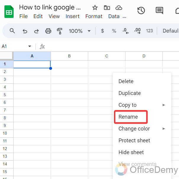
Press the right click of the mouse on the sheet icon for which you want to rename, you will have a “Rename” option through which you can change the sheet name.

Step 2

Now, simply write the name of the sheet that you want to give and press the “Enter” key. The sheet name will be changed.

Conclusion

It is not the end, there are so many related topics that may be helpful to you can explore with Office Demy, so go through our website and share your opinions in the comment section Also tell us how you find the above article on how to link Google Sheets together.