
To use AND Function in Google Sheets
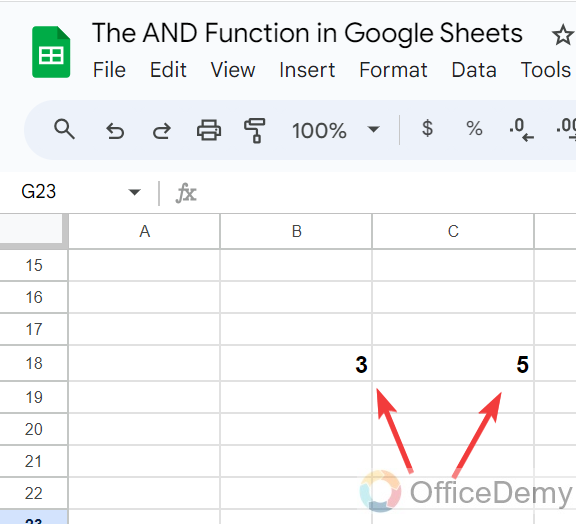
- In a cell, enter your data (e.g., B18 = 3, C18 = 5).
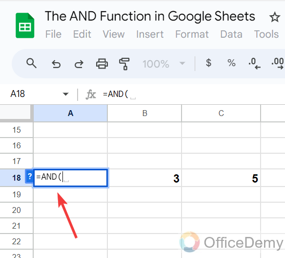
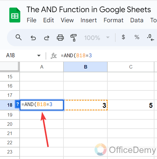
- In another cell, start the AND function by typing =AND(Enter the first logical expression (e.g., B18=3).
- Add a comma.
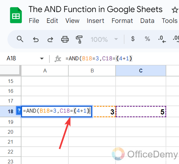
- Enter the second logical expression (e.g., C18=(4+1)) > Close the function with ).
- Press Enter.
- The result will be “TRUE“
OR
- Create data with text strings.
- Start the AND function in a cell.
- For logical expressions, use cell references and text in quotation marks > e.g., =AND(A2=”Text“, B2=”Example“).
- Press Enter.
- The result will be “TRUE” if both conditions are met.
Today we will learn the complete AND Function in Google Sheets. No doubt! Google Sheets has plenty of functions and features that make your tasks more effective. One of the functions, The AND function in Google Sheets is also in the list. The AND function in Google Sheets is a logical function that checks whether the value is true or false. When all values are true then it will give you a true value but if any one of the given expressions is false it will give you false.
Today, in this tutorial on the AND function in Google Sheets, we will discuss some examples regarding the AND function to learn how it works but first let’s see the advantages of this function in the next section.
Benefits of the AND Function in Google Sheets
The AND function is used to check the values that all given expressions are fulfilling the criteria simultaneously or not. You may usually need to evaluate logical expressions collectively and determine whether all conditions are met, in such a situation the AND function in Google Sheets is most useful to you.
Syntax
=AND(logical_expression1, logical_expression2)
How to use AND Function in Google Sheets
In this step-by-step guide to the AND function in Google Sheets, we will overview two different examples to learn how can we use the AND function in Google Sheets.
Example # 1: Simple usage of the AND function
In this method, we will simply use the AND function between the values in Google Sheets.
Step 1
Let’s suppose, we have two different values in different cells as written in the following sample data. Let’s see how we can find value is either true or false with the help of the “AND” function of Google Sheets.
Step 2
Place your cursor in the cell where you want to find that the value is true or false and start the “AND” function by just writing AND with an equal sign.
Step 3
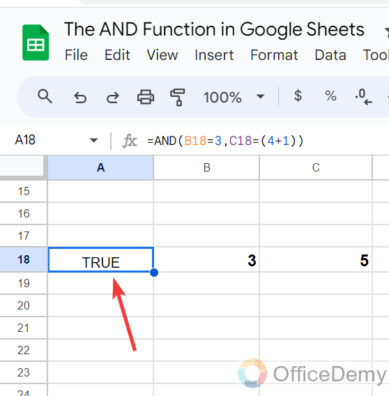
After starting the AND function, we will give the first logical expression according to the syntax as here I have written “B18=3” in the syntax.
Step 4
Similarly, after giving the first logical expression, we will then specify the second logical expression. You can also write your logical expression in the following pattern as I have written “C18=(4+1)” which is equal to “5“.
Step 5
As the cell B18 contains “3” and C18 is equal to “5” it means, both given logical expressions are true so here we have gotten the result “TRUE” as directed below.
Example # 2: Using AND Function Between the Text String
In this method, we will learn how to check values when there is a string in the dataset with the help of the AND function in Google Sheets.
Step 1
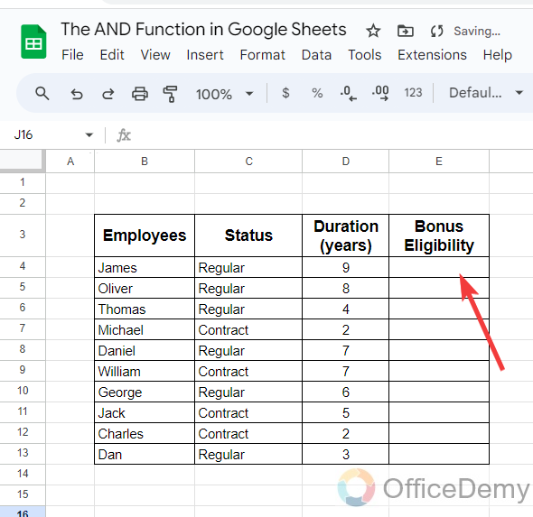
In the following sample data, as you can see below, we have some string text in the data in which we need to check if the value is true or false. Let’s see how we can find it with the help of the AND function.
Step 2
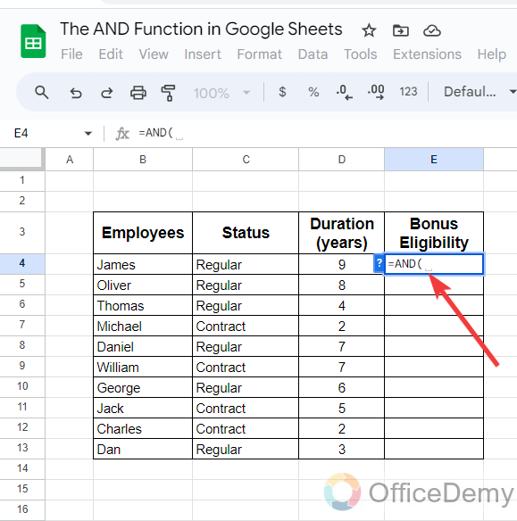
Simply run the “AND” function of the Google Sheets in the cell where you want to get the result as written below.
Step 3
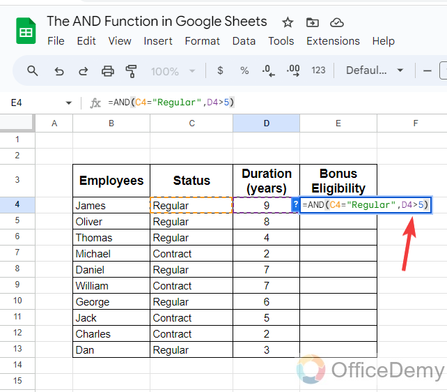
To give the logical expression of the text in Google Sheets, first, you will give the cell reference and then write the string in quotation marks as I have written in the following screenshot.
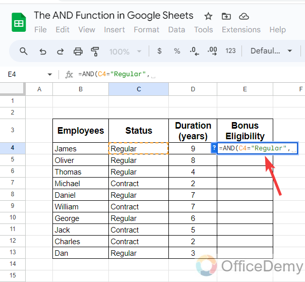
Note: Make sure that you are writing the correct spelling of the string to get the true value.
Step 4
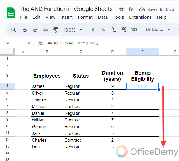
Now simply give the second logical expression of the syntax according to your data and then press the Enter key to get the result.
Step 5
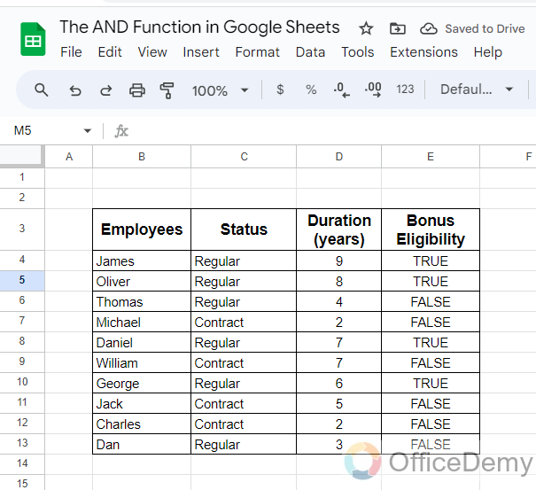
When you press the Enter key you will get your result in true or false as I have gotten below, now just simply drag this formula over the other cells to get all results.
Step 6
In this way, you can check the value if true or false even within text string data in Google Sheets with the help of the AND function.
Frequently Asked Questions
Can I Use the AND Function in Google Sheets to Insert a People Chip?
Yes, you can use the AND function in Google Sheets for people chip integration. This handy feature allows you to combine multiple conditions using the AND operator to create more complex formulas. By integrating people chips, you can streamline data entries, making your spreadsheets more efficient and collaborative.
How to use the AND function with the OR function of Google Sheets?
Although you can also check multiple conditions by using the AND function of Google Sheets if you have complex logical conditions in your dataset then you may check if any of the specified conditions are true by the combination of OR and AND function of Google Sheets. Let’s look at a practical example of nesting of AND and OR functions in the following steps.
Step 1
In the following sample data, if you see here, we have three different scenarios to see whether the value is true or false. In such a situation we can use the combination of OR and AND function of Google Sheets.
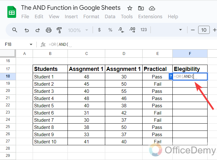
Step 2
To nest the OR function with the AND function in Google Sheets, first we will write the “OR” function of Google Sheets with an equal sign then will add the “AND” function in the syntax after the small bracket as written below.
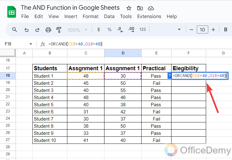
Step 3
After starting the “AND” function of Google Sheets, we will complete the arguments of the AND function by writing the first two conditions as I have written in the following picture.
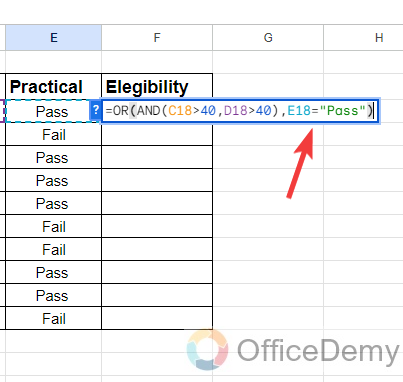
Step 4
After writing the first two logical expressions close the bracket and then specify the 3rd logical expression of the dataset into the syntax as directed below.
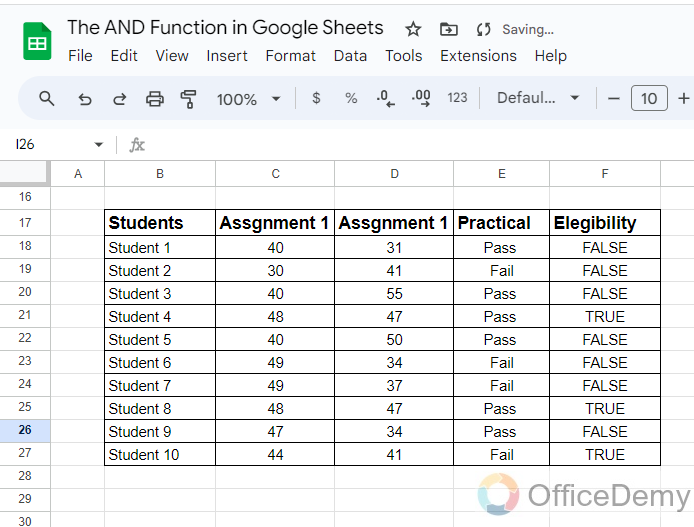
Step 5
Once you have completed the syntax drag the formula over the other cells after getting the first result. In this way, you can check whether the value is true or false between multiple values as well.
How to use the AND function with the IF function of Google Sheets?
As you know when we check the value is either true or false with the help of the AND function, it gives the results in the form of TRUE and FALSE but with the help of using the IF function with the AND function, we can specify any other values instead of TRUE and FALSE by inputting in arguments. When we use the IF function with the AND function of Google Sheets, TRUE and FALSE automatically turn into the specified values. Let me show you practically in the following step-by-step guide, how to use the AND function with the IF function of Google Sheets.
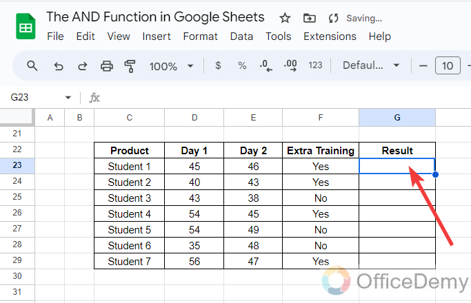
Step 1
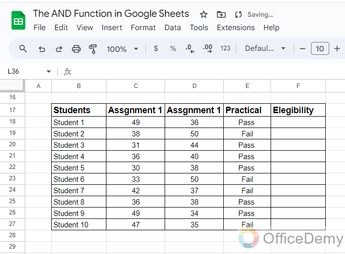
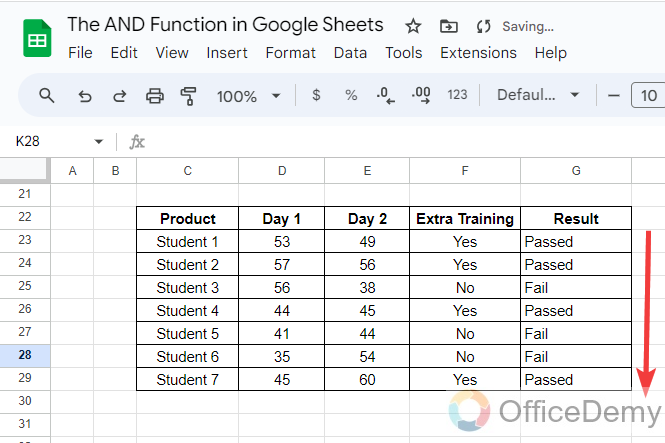
In the following sample data, we have three different criteria, which we want to label “Passed” or “Fail” for those students who are fulfilling the criteria. Let’s see, how we can do it with the help IF+AND function of Google Sheets.
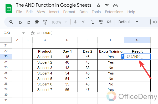
Step 2
First, we will start the IF function in the cell with an equal sign, then will run the AND function of Google Sheets after placing the small bracket as can be seen below.
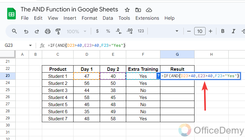
Step 3
After starting both functions, write all conditions that are required in the syntax as I have written in the following picture.
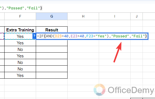
Step 4
Once you have written all the logical expressions, close the bracket and then write the values that you want to get in return when it is true or false as I have written “Passed” and “Fail” in the following syntax.
Step 5
Once you have written the syntax, then press the Enter key to get the result. To get the other results just drag the formula over the other cells as you can see the result in the following picture.
Conclusion
In the above article on the AND function in Google Sheets, we have covered all the things that you should know regarding the AND function in Google. Hope it will be helpful to you.


