Google Sheets Formulas Tips & Techniques You Should Know

If you know all the functions and formulas of Google Sheets and think that you are a Professional of Google Sheets then you are wrong, A True Professional must know the hidden, little tips and tricks and shortcuts of Google Sheets. So here Office Demy has brought to you several Google Sheets Tips and techniques you should know that can make you more effective in Google Sheets.

Advantages of Google Sheets Tips & Tricks

These little tips and tricks are not as mean but if you combine them and if you become handy with them then it can give you a big boost in your functionality of Google Sheets. It saves a lot of time and effort and gives you effective and efficient results when you are working with Google Sheets. So, let’s go towards the next section to learn Google Sheets tips and techniques that you should know.

1- Absolute Cell

Absolute cell or reference in Google Sheets in which the columns and rows stay constant while copying a formula from one cell to another cell. To absolute cell reference, we use the “$” sign between the ranges but you can absolute any cell reference by just clicking the “F4” key instead of writing the “$” sign.

It is the most useful shortcut used in Google Sheets. Just place your cursor along the cell reference and press the “F4” key, and the range will instantly be absolute as can be seen GIF below.

2- Edit cell

Secondly, I will talk about the most useful activity of Google Sheets is the Edit cell. Most users are not aware of the shortcut key to edit a cell, they usually press the enter key to edit a cell and they fail because the shortcut key to edit a cell is “F2” which is most useful as well.

Especially, when you have applied a formula in the cell and you want to update it then just place your cursor over the cell and press the “F2” key, and your cell will be in edit mode.

Similarly, when you have to edit a text into the cell then you don’t need to even touch the mouse just move the cursor over the desired cell by arrow keys and then press the “F2” key you will be in edit mode as I have edited a cell in the following GIF.

3- Exit Formula

Let’s suppose, you want to edit a cell, but accidentally you mess up with any applied formula that doesn’t need to, in such a situation there is a shortcut key “Esc“.

Pressing the Esc key not only closes the formula but also discards all the changes that have been made accidentally and gives you the cell in its previous form.

This tip would be very helpful to you because most users make mistakes while working on a sheet in a hurry, it can prevent you from any loss of data in cell or formula errors.

4- Display Formula as a Text

When you need to write a formula in the cell, you need to place an equal sign along it, which causes the function to run. In this case, you are unable to write a function formula as a text string in the Google Sheets cell.

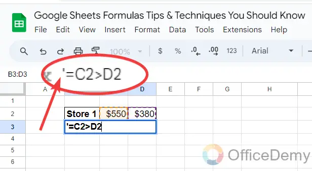
Don’t worry I have the solution to your problem, just attach an apostrophe before the function to display a formula as a text string. Let me show you practically in the following steps.

Here, as you can see in the following GIF, I am writing a formula that I want to display as a text string, but it is showing me a result. Let’s see how we can display this formula as a text string.

Just write an apostrophe sign before the equal sign as I have written below.

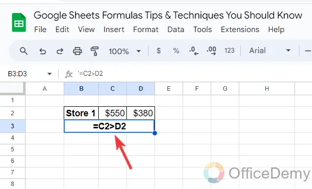
Inserting an apostrophe sign will turn your formula into a text string as can be seen in the result below.

5- Formula Helper Pane

Google Sheets is very familiar to its users because of its finest guidance. Even a new user can easily understand its formulas and functions with the help of the following trick.

If you are a new user of Google Sheets and applying formulas in your spreadsheet documents that are unable to understand you or you have forgotten any argument, or parameter for a formula then you can click on the following highlighted help icon for the formula.

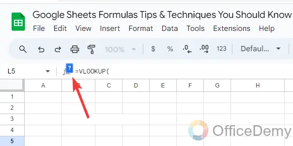
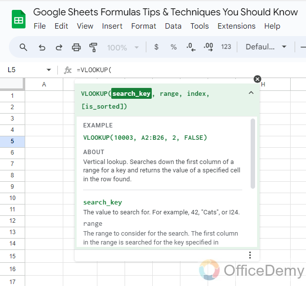
This help icon will give you a formula helper pane through which you can easily insert all arguments regarding any function of Google Sheets. This formula helper page will provide you with complete details for every single argument regarding function in Google Sheets.

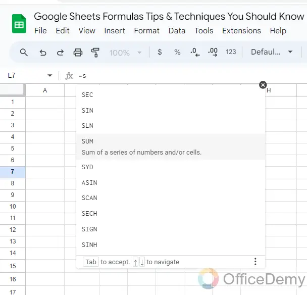
6- Formula Suggestion Drop-down

As I have discussed above, Google Sheets is very familiar to its users due to its easy guidance. Let’s suppose you are new to Google Sheets but have forgotten the function that you need to apply then there is nothing to worry about, just write the first letter of the function in the formula bar, and it will show you all the functions regarding specific letters.

This is a great and tricky way to discover a function in Google Sheets.

7- Tab to Select Formula

Tips & tricks make your tasks more efficient, similarly, this trick can also save you much time and effort while working on a sheet. As we have learned above, to discover a function by just writing a letter this trick is to select the function when you have discovered it.

As you can see practically in the following animation, write the first letter of the function once you have found your desired function, go on the function, and press the “Tab” key that function will run automatically in the cell.

8- Adjust Column Width

Working with Google Sheets is always challenging due to its cell boxes, it becomes difficult to organize text into cells because sometimes cell size becomes very large against text and sometimes text goes out of the cell.

In such a situation follow the following instructions to organize your cells by fitting with the text you can do this by just double-clicking on the edges of the column that will fit the column width according to the text in the cell and give you organized data.

9- Aggregation Toolbar

The Aggregation toolbar is a great facility for analyzing data for the short term. For example, if you are monitoring a huge amount of data in which you need to know the sum, average, max, min, and count of selected values then you can quickly take an overview of the selected cell.

As you can see in the following example, we have selected a range for which you can see its Sum value, Average, Max, and Min value from the aggregation toolbar at the right bottom of the Google Sheets.

10- Quick Fill Down

It is most useful to fill down the range in Google Sheets when you want to find the same result for a range then you don’t need to write the same formula on every cell even if you don’t need to copy the formula over the cells just double click on the small blue square along the cell selection, it will quickly fill down the range as resultant below.

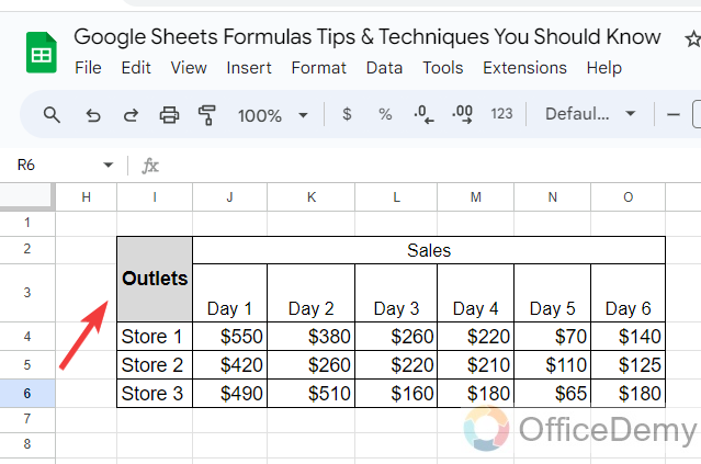
11- Wrap Text

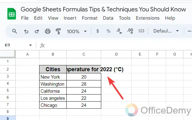
Google Sheets consists of cells in which we write the text for working, these cells have a standard size and write text in a single line. But if you want to write text in multiple lines in a cell then you may need the feature of “Wrap text” in Google Sheets.

For example, here a text is going out of the cell that is in one line. Let’s see how we can write in multiple lines.

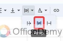
Look into the toolbar of Google Sheets, you will find the “Wrap text” option icon as highlighted below. Click on it to wrap the text.

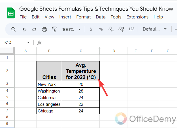
Clicking on the Wrap text icon will turn your text into multiple lines as result below.

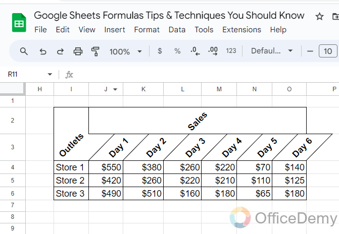
12- Text Rotation

Google Sheets also offers plenty of options to format the text more than coloring and styling the text. In the tool Google Sheets, you will find the following icon through which you can rotate your text in the cell to provide a stylish preference as per need in the dataset.

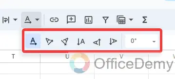
Just select the alignment of rotation, and your text will rotate in the selected rotation as a result below.

13- Format Painter

If we are talking about tips and tricks for Google Sheets, then how can we forget the “Format Painter” tool of Google Sheets? It helps when you want to apply the same formatting over multiple cells.

Let’s suppose, you have formatted a cell as seen below, now you want to apply the same formatting over the other cells as well.

Then simply, simply select the cell, take a ruler from the Format Painter icon, and lap over the other cells. They will instantly be formatted the same as first.

14- Slicer

Slicer is used to filter data in specific values or ranges in Google Sheets. To apply a slicer in Google Sheets just go into the “Data” tab and click on the “Add a Slicer” option as highlighted below.

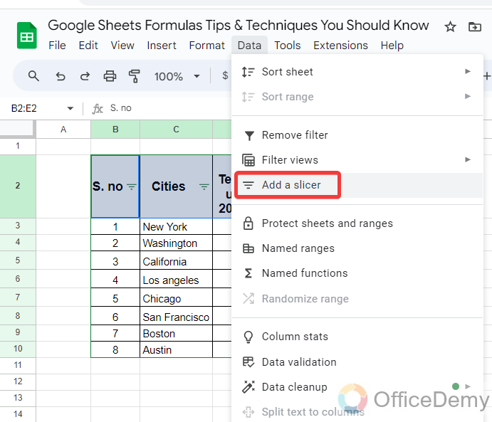
If your table has multiple values data, you can filter it according to your need with the help slicer I needed just the data for “Austin” and “California” so I have filtered them with the help of the slicer in the following example.

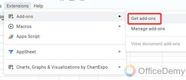
15- Add-ons

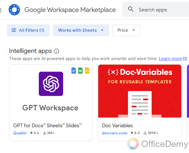
Google Sheets is becoming a vast application for spreadsheet documents, but still, it is unable to accomplish most of the tasks regarding spreadsheet documents. But in such a situation you can use additional tools in Google Sheets called “Add-ons“. You can access these “Add-ons” from the “Extensions” tab of the menu bar.

The following window will open in front of you, where you can find a tool regarding your tasks and can easily install it to accomplish your tasks in Google Sheets.

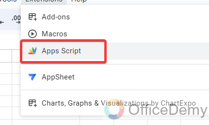
16- App Script

The Apps Script allows you to add JavaScript and HTML-based code that can define and handle custom functions. You can access it by clicking Extension and then selecting Apps Script.

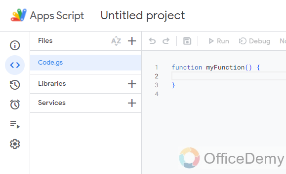
When you click on the “App Script” option it will give you a new separate window as follows where you can create your function for Google Sheets.

Conclusion

I am 110% sure that most of the above tricks you were not aware of but know you because Office Demy always takes care of the professional building of its users and makes them more efficient regarding office solutions. For more similar topics like Google Sheets tips and techniques, you should know to keep visiting Office Demy.