How to Use OR Function in Google Sheets

Today we will learn how to use the OR function in Google Sheets. The Or function of Google Sheets is a logical function that checks the values and gives us the value in return True or False. In this article on the OR function of Google Sheets, we will discuss how to use the OR function of Google Sheets. So, let’s get started.

Benefits of the OR Function in Google Sheets

We use the OR function to check the values in the data. This logical function gives you TRUE and FALSE responses, which you can use to sort through your data. You can also add the OR function with the AND function to find the value in return in multiple scenarios. The combination of the OR function with the IF function gives you the desired string instead of True and False. Let me show you practically with the help of examples in the following section of a step-by-step guide on the OR function of Google Sheets.

How to use OR Function in Google Sheets

In this tutorial on the OR function of Google Sheets, we will do a practical of two different uses of the OR function of Google Sheets.

Use Case # 1

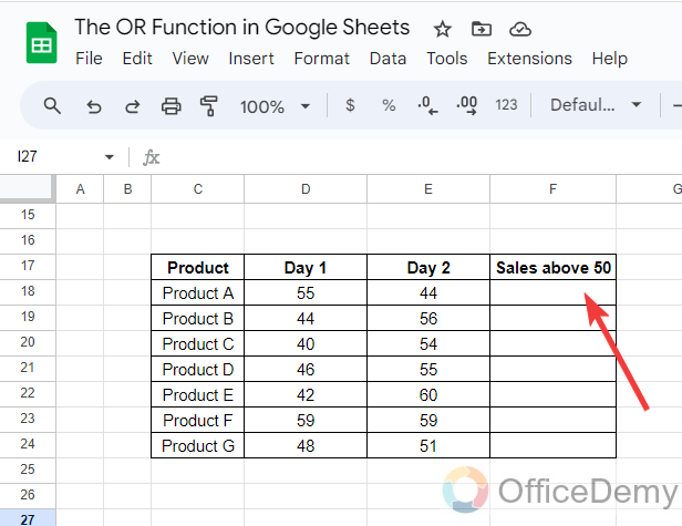
Step 1

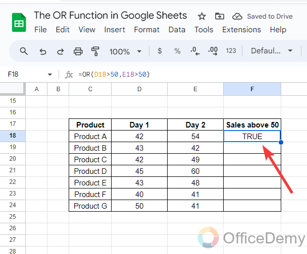
If we look at the following example, we have sample data of sales for a couple of days for some products. Here we will find that any sale is greater than 50 items in a day by using the OR function of Google Sheets.

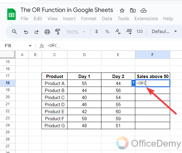
Step 2

First, place the cursor where you want to apply the OR function of Google Sheets and write the “OR” with an equal sign in the cell to start the function as written below.

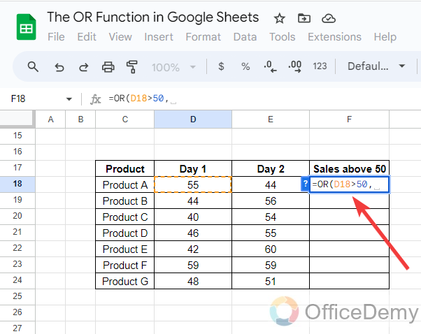
Step 3

According to the syntax of the OR function, first, we will specify the first logical expression as here I have written that “D18>50” as the first expression of the function.

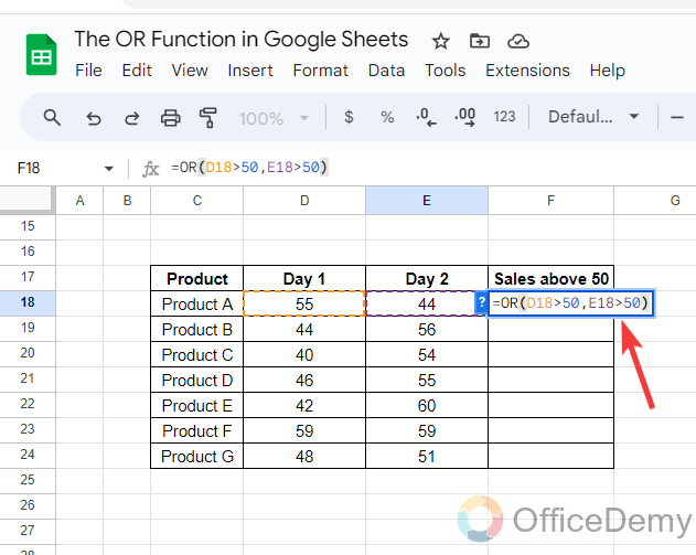
Step 4

In the same way, now we will specify the second logical expression, as here we are looking for sales greater than 50 so here as well, we have written “E18>50” as can be seen below.

Step 5

In this example data we have only two criteria so here we will close the function and press the Enter key to get the result as I have gotten in the following picture.

Step 6

Once you have gotten the first result in the cell then you can get all other results by just dragging the formula over the other cells as directed below.

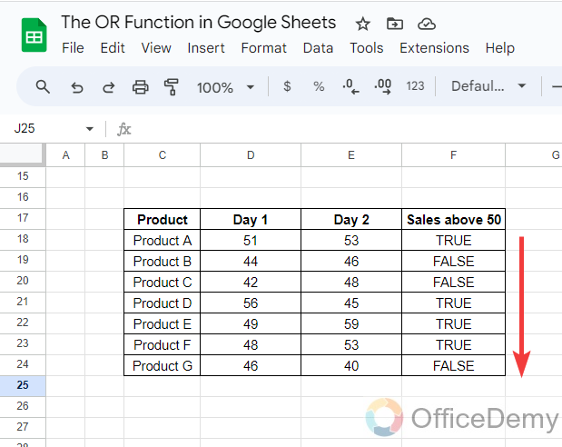
In this way, you can check the result whether the value is true or false by using the OR function of Google Sheets.

Use Case # 2

Step 1

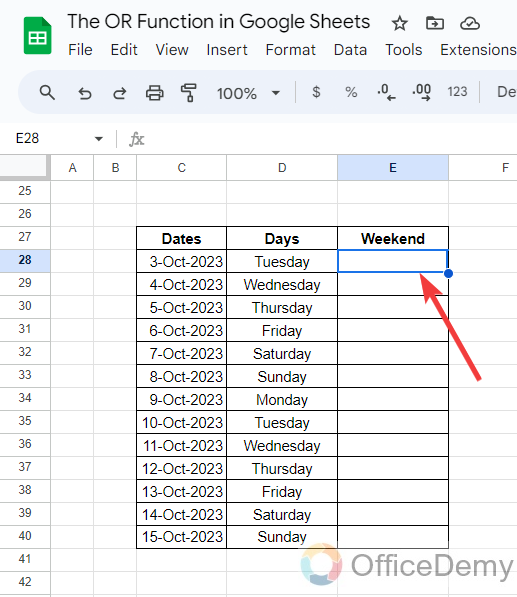
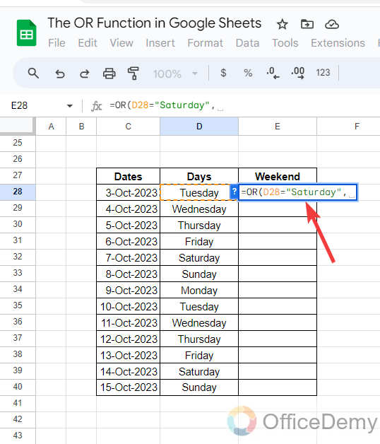
In the following example data, we have the string for weekdays in the column as can be seen below. We need to check whether any weekend is present by using the OR function of Google Sheets.

Step 2

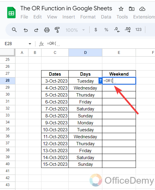
Similarly, in this method, we will write the first part of the syntax which is the function name to run the function as I have started in the following example.

Step 3

After starting the function, we will specify the first condition that we are looking for. Here I have written “D28=” Saturday” to find the “Saturday” from the list.

Step 4

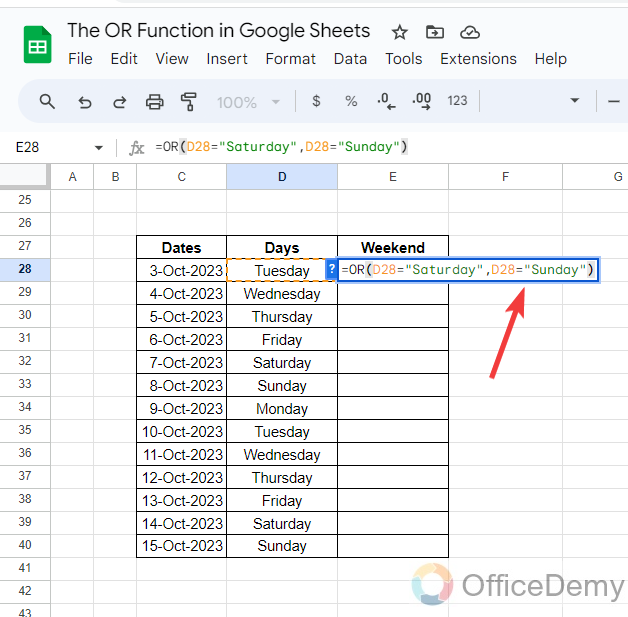
As you know the second weekend day is “Sunday” so here we have specified the second condition to look for Sunday in the data by writing “D28=”Sunday” as written below.

Step 5

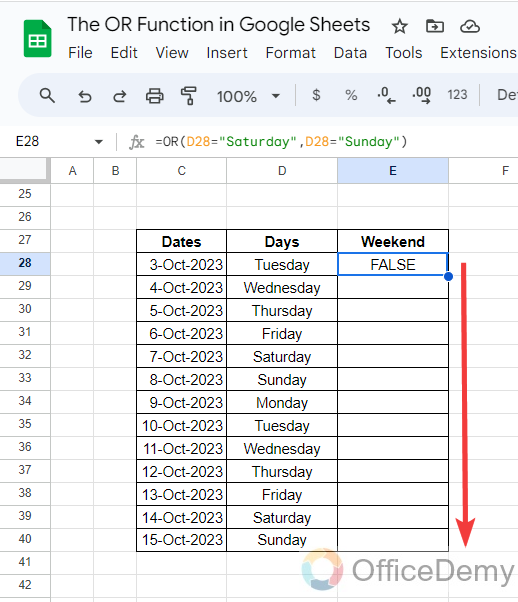
Once you have completed the syntax press the Enter key to get the result, then drag this formula over the other cells along the weekdays to find weekend days in the data.

Step 6

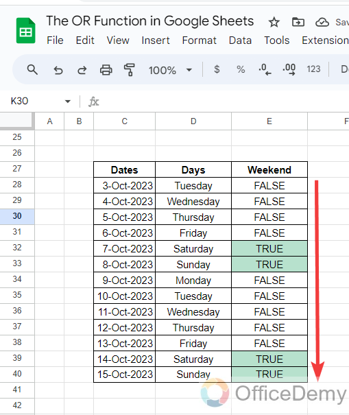
The result is in front of you that the cells that are equal to “Saturday” and “Sunday” are indicated by “True” as highlighted below. In this way, you can find whether there are weekend days in the data.

Frequently Asked Questions

Can the OR function be used in conjunction with the IMPORTXML function in Google Sheets?

The google sheets importxml function does not support the OR function directly. However, you can use multiple IMPORTXML functions within an IF function to achieve similar results. By nesting the functions, you can set up conditions and fetch the desired data from multiple sources.

How to use the OR function with the AND function of Google Sheets?

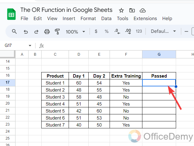
In the OR function of Google Sheets, we can give only two logical expressions from the data range. Still, if you need to specify more conditions in the syntax to check whether true or false then you will have to use the OR function with the AND function to give multiple conditions. Below are the steps through which you can easily understand practically.

Step 1

In the following data, we have three different scenarios with the help of which we will check whether the student is eligible for passing criteria or not with the help of a combination of OR and AND functions of Google Sheets.

Step 2

First, we will write the “OR” function with an equal sign to start, then run the “AND” function after adding the small bracket in the syntax, as seen in the following picture.

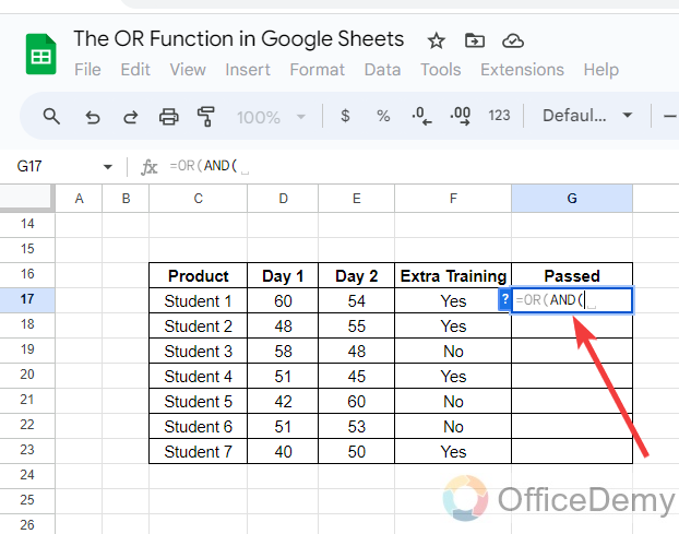
Step 3

After starting both functions, first, we will write the values of the “AND” function of Google Sheets to complete it where I will specify the first two conditions as directed in the following screenshot.

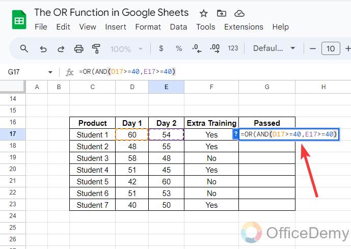
Step 4

Once you have written the first two scenarios of the data, then close the bracket to close the AND function then write the third condition of the given data as written in the following picture.

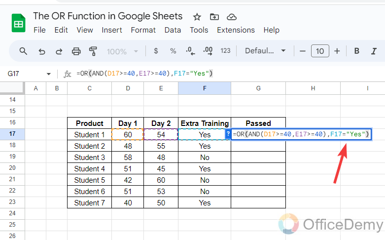
Final Formula: =OR(AND(D23>=40,E23>=40),F23=”Yes”)

Step 5

Once you have completed by giving both expressions for both functions then simply press the Enter key to get the result, after getting the result drag down the formula over the other cells to get the other results.

Here you can see the result in the following picture that the ranges that fulfill the given criteria come true and the rest are false.

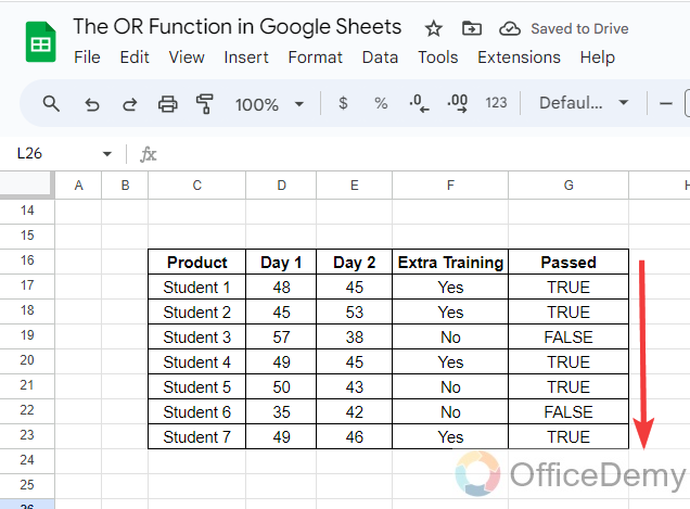
In this way, you can check whether the value is true or false in multiple conditions by using the combination of OR and AND function of Google Sheets.

How to nest the IF function with the OR function in Google Sheets?

When we apply the OR function of Google Sheets, it gives us the result in True or False only but if you want to get any other values in the place of True and False then you may need to nest the IF function with the OR function in Google Sheets.

Step 1

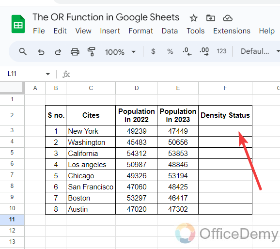
In the following data, here we have a table of different cities with the population of two different years. In this table, we will check the density status of the population for these cities and label it with high density or low density with the help of the nesting IF function with the OR function of Google Sheets.

Step 2

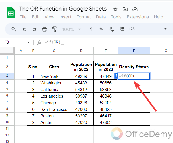
First, we will write the “IF” function of Google Sheets and then add the “OR” function in the syntax in the following pattern I wrote in the following picture.

Step 3

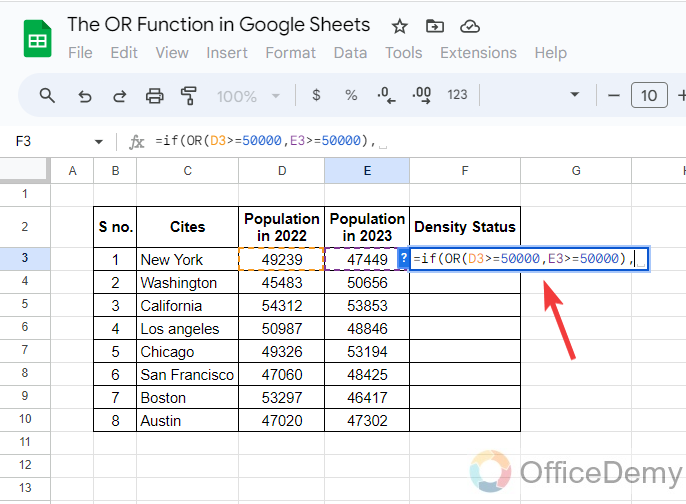
According to the OR function, here we will specify the criteria that we want to look for here I am checking if there is any value greater than 50 thousand, so we will write the formula in the following way as written below.

Step 4

After giving the criteria our OR function has been completed, now we will specify the value in return according to the IF function here I have described “High Density” and “Low density” as true and false respectively as highlighted below.

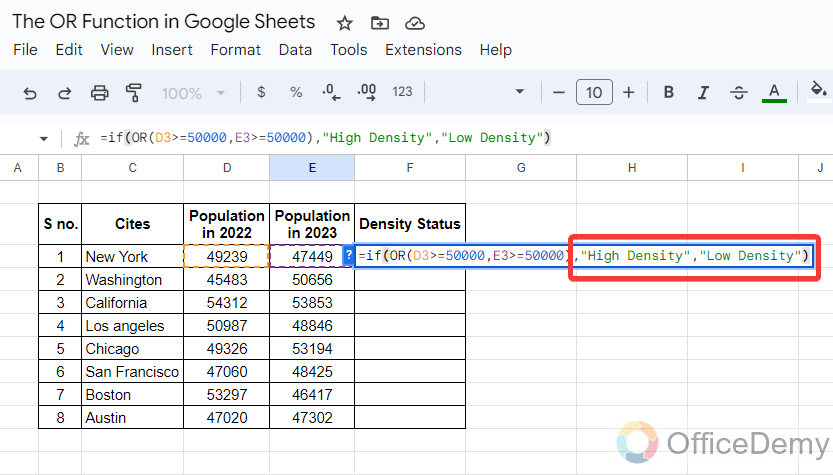
Final Formula: =if(OR(D4>=50000,E4>=50000),”High Density”,”Low Density”)

Step 5

Once you have completed writing the syntax simply press the Enter key to get the result, then drag the formula over to the other cells. You will get the result as follows.

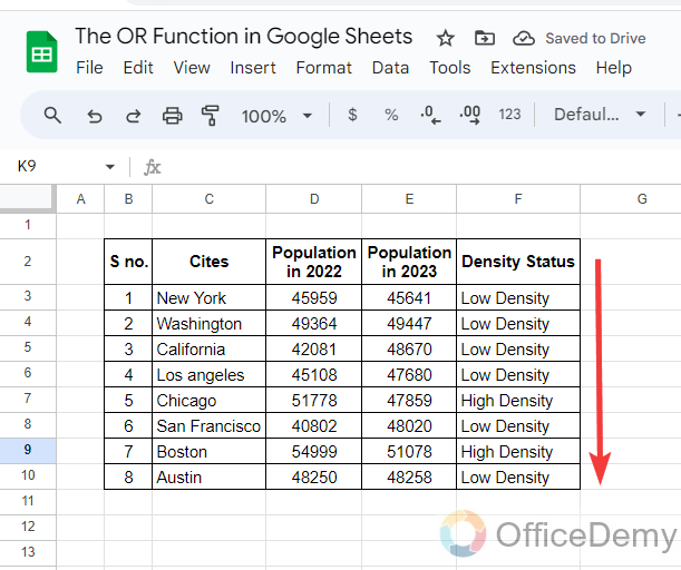
In this way, you can not only check whether the value is true or false, but also can label it with a specified string.

Conclusion

In the Google Sheets, you may need to check if it meets specific criteria where the OR function in Google Sheets can be very helpful to you that we have learned in the above tutorial, we have also covered the usage of OR functions with other functions that will be beneficial for you. Thanks and keep learning with Office Demy.