
To Use Filter Function in Google Sheets
Using a Single Condition:
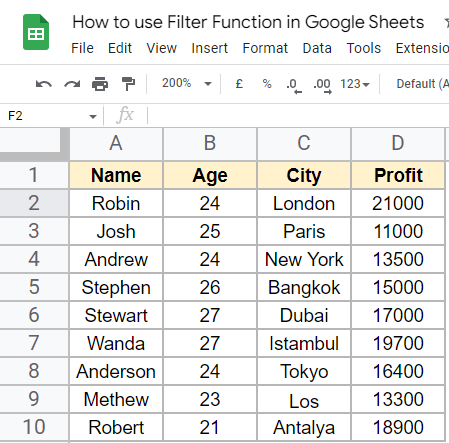
- Select a sample dataset.
- In a cell, start the formula with =FILTER( > Specify the data range as the first argument.
- Add your single condition.
- Hit Enter to get the filtered results.
Using Multiple Conditions:
- Follow the same steps as in Method 1.
- Add a comma and write another condition.
- Hit Enter to filter data based on multiple conditions.
Using Other Functions:
- Begin with the FILTER function and specify the data range.
- Select the column to filter.
- Use a mathematical function (e.g., B2:B10>AVERAGE(B2:B10)) to filter data based on a calculated value.
- Press Enter to get the filtered results.
Tip: Learn more methods in the article below.
Hello, welcome to another article. In this article, we will learn how to use the Filter function in google sheets.
The filter function as the name suggests used to filter the data. But, it’s not this simple. The filter is one of the most powerful functions in google sheets. Its dynamic function means that if the source data is changed, then the result will also be affected. The filter function can be used in hundreds of possible ways using various conditions, and combinations of the conditions. we can use other mathematical functions within the filter function, and also, we can use the conditional statements link AND and OR. Let’s move forward and learn in detail.
Use cases of Filter Function in Google Sheets
We often work with data ranges that are huge and have a lot of combinations of data that can be filtered to analyze the data from many aspects to determine handy insights. The filter function can be the one that is used for filtering the same data set in many various ways using different functions and logic. It gives us actual insights into the data that cannot be analyzed manually. Therefore, we need to learn the filter function. Another reason is that the function is dynamic, which means we can create real-time dashboards using the filter function and drop-downs in google sheets.
How to use Filter Function in Google Sheets
From this section we will see various use cases to use the Filter Function, first, let’s see the syntax then we will move on to learn how to use the filter function in google sheets.
=FILTER(range, condition1, [condition2, ..])
- range: The source data range you want to filter using the Filter function.
- condition1: A data range row or columns correspondent (this should be an equal number of rows as your source range has). It returns a Boolean value based on the condition.
- [condition2]: This is an optional argument, it is the second condition to use when using OR, AND, and other logical conditions. This also should be equivalent to the previous argument (the number of rows should be equal). It also returns a Boolean value based on a given condition.
How to use Filter Function in Google Sheets – Using A Single Condition
In this first section, we will learn how to use the filter function with a single condition. This is going to be the basic usage of this function. For this, we will need some data to work on. So, see the below steps and follow me with the example.
Step 1
A sample dataset
Step 2
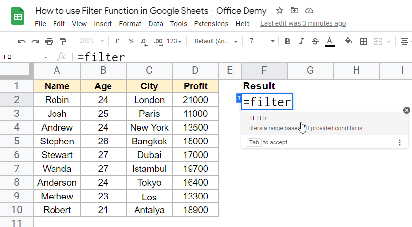
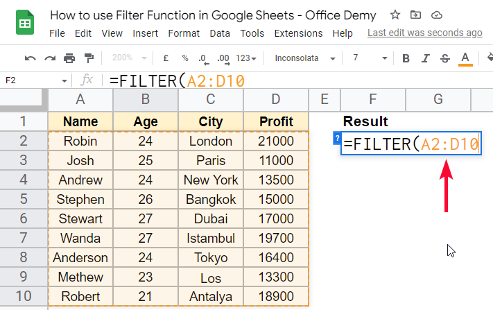
In any other cell, write the filter function starting with “=”
Step 3
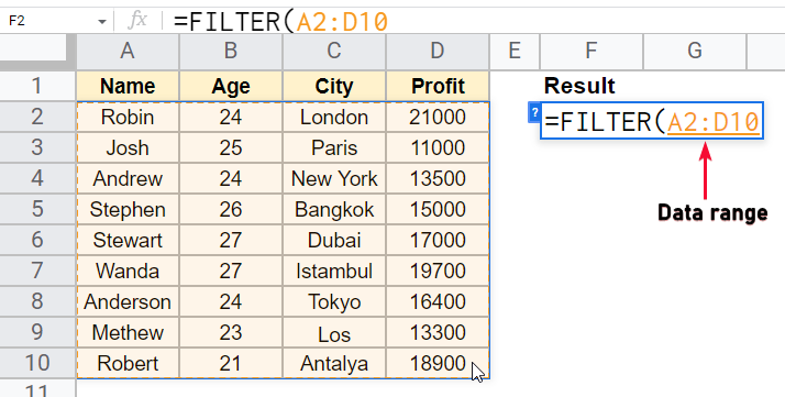
Pass the data range as the first argument.
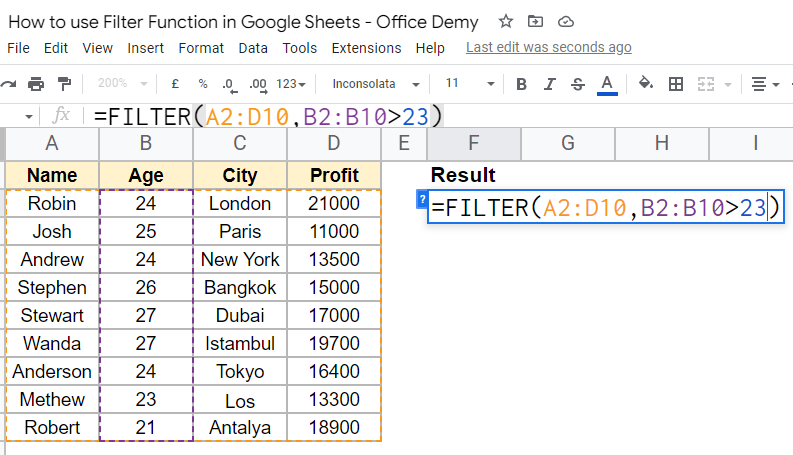
Step 4
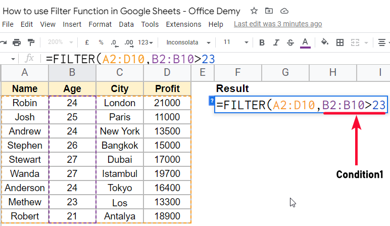
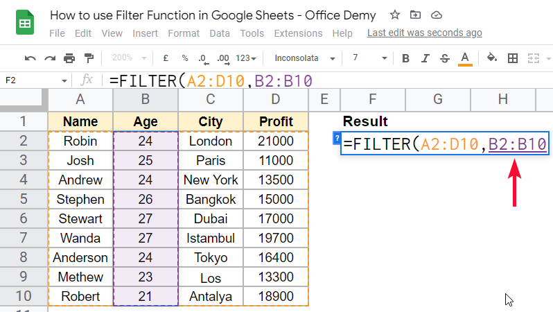
Pass the condition1
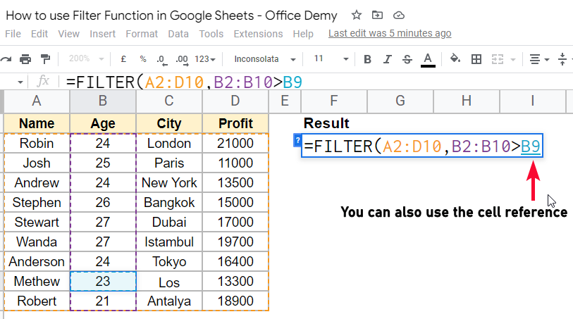
Step 5
You can hard-code the value, or you can pass the cell reference of that value
Step 6
Hit Enter key, and you got the result
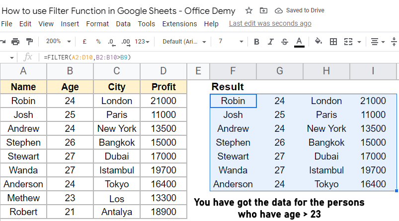
This is how simply you can filter out anything from the dataset based on a single condition.
How to use Filter Function in Google Sheets – Using Multiple Conditions
In this section, we will learn how to use the filter function in google sheets using multiple conditions. We had a condition in the previous section where we filtered out the data of a person having an age greater than 23, with the same condition we can add another condition such as age is greater than 23 and the profit is greater than 15000. This can be simply done following the below steps.
Step 1
Write the formula same as the previous
Step 2
Add a comma, and write another condition
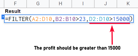
Step 3
Hit Enter key and you’re done.
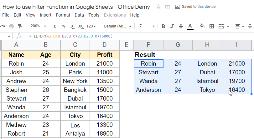
Note that whenever you compare a column in a condition inside the Filter function, you select the entire column (excluding headers) to match the number of rows with the sort data, here my source data has nine rows, so in every condition when I compare any column, I will have to select the whole column. If the number of rows is unmatched, you will get an error.
Now let’s move forward and learn the Filter function with some complex use cases.
How to use Filter Function in Google Sheets – using OR Condition
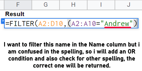
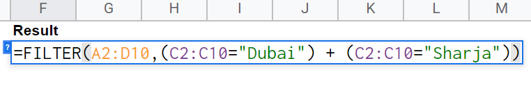
In this section, we will learn how to use Filter Function in Google sheets with OR condition, we have already seen the AND condition in the second method where we learned to add two conditions. To use OR condition we need will utilize the same example. Let’s say I want to check the Name section and find out any name, and then I will add another condition where I will add another name, because I am not sure about the name, so I will pass two possible names and the correct one will be returned.
Step 1
Filter anything using a simple single condition method.
Step 2
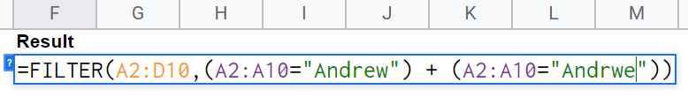
Add a + sign, and research for a similar data point for which you are not sure
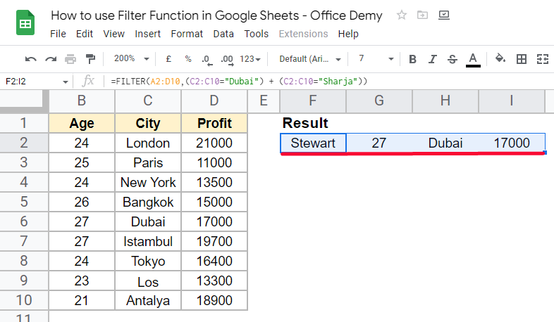
Step 3
Hit Enter key, and you will see the correct value will be returned from two defined values.
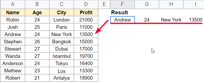
This is how OR logic works, using the same logic you can make hundreds of use cases to filter the data.
How to use Filter Function in Google Sheets – With Other Functions
In this section, we will learn how to use the Filter function in google sheets with other functions such as average, max, min, etc.
This is another common use case where we need to have the value based on a mathematical calculation, so the filter function helps us and solve this problem in a single step, we don’t have to find the average separately then pass it inside the Filter function, we can do both steps inside Filter function.
We will use a simple use case to understand how it works. We make nested functions inside the filter function. Let’s see how it’s done.
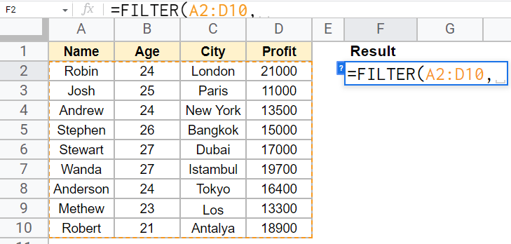
Step 1
Write the Filter function and pass the entire dataset
Step 2
Pass the column from which you want to filter the data
Step 3
Now I want the values that are greater than the average value, so I don’t need to calculate the average value first instead I can use the following syntax.
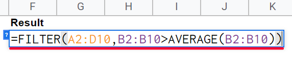
B2:B10>AVERAGE(B2:B10))
The above statement says that find filter values from B2:B10 only when the value is greater than the average value of B2:B10.
Step 4
Press Enter, and you have got the result
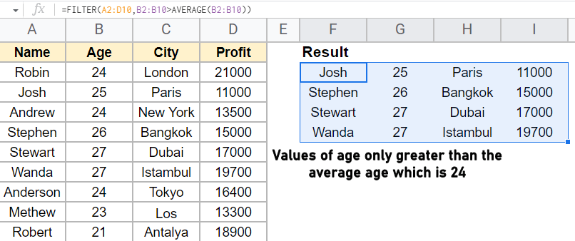
This is how we can use other functions inside the Filter function to make a shorter syntax and perform some complex tasks.
How to use Filter Function in Google Sheets – to Filter Top 3 & Top 5
In this section, we will learn how to use the Filter function in Google Sheets to Filter the top 3 & top 5.
We can bring top (any number), there is no limitation but the number should be less than the number of rows of the source data.
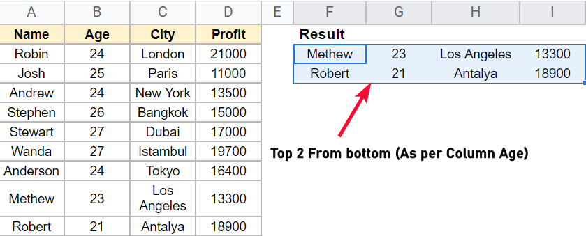
We can find the top 3 or top 5 from above, and also from the bottom.
Step 1
Write the filter formula and pass the entire data range
Step 2
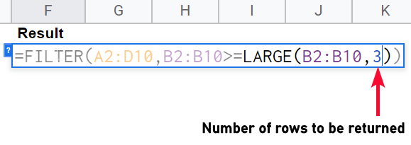
Just like we used the average formula in the previous section, here use the Large function with a condition “greater than equal to” for the upper top 3 or 5.
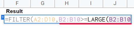
Step 3
Pass a number 3, or 5, or any number to define how many rows you want to return.
Step 4
Hit Enter key, and you have got the result
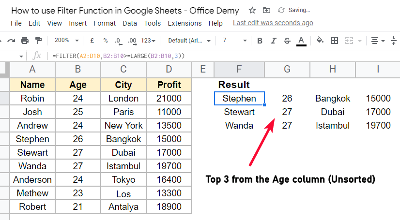
Note: We can SORT the filtered data using a sort function
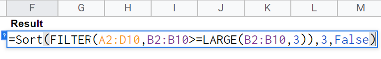
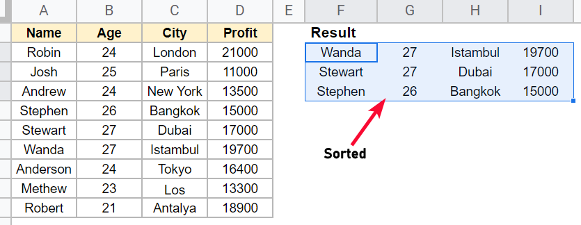
This is a logic in which we compare the large values inside a column and give a number to specify how many rows to return.
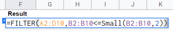
To find the same data from the bottom we will use the Small function.
Only Step
Use the Function Small instead of Large, and change the condition to “less than equal to”.
Hit Enter key and you have got the top values from the bottom.
How to use Filter Function in Google Sheets – Making a Mini Dashboard
Using a dropdown list, a chart, and a filter function, we can make a simple dashboard like the below.
Download/Copy Google Sheets Practice Workbook
Get a free template and make a copy to play around with. Be experimental and explore new features.
Important Notes
- The Filter function is dynamic. If the source data is changed, the resultant cell will also change according to the effect of change.
- The filter function returns an unsorted range
- The filter function can be used with more functions, try it out and make your logic
- The filter function can be used with many other functions
- It returns an Array value, which can show up as an error if there is already something existing in the cells in which the array needs to be spread. It will not overwrite the data, instead, it will show up an error so you can manually remove your already written data that is overlapping the array value result
Frequently Asked Questions
What are the Different Ways to Filter Data in Google Sheets?
Google Sheets offers various filter functions in google sheets to help users sort and organize data effectively. By utilizing these filter functions in Google Sheets, users can easily rearrange their datasets based on specific criteria. Whether it’s filtering by date, text, or numbers, these functions provide a seamless way to narrow down the information and focus on what’s relevant. With just a few clicks, users can refine their data and make it more manageable for analysis and decision-making.
How filter function works dynamically?
Assume you have 4 columns in your data that show the profit of four different months, now in a cell you can create a drop-down having all four values. Now you add a filter function in which you passed the reference of the cell in which your dropdown exists. Now on the change of the value, each time in the drop-down cells the values of the data coming from the Filter function will automatically update every time. This is called the dynamic behavior of the Filter function. As we have done in the above section.
Conclusion
Wrapping up how to use the Filter function in google sheets. We have learned this function in every detail. The filter function is very commonly used along with the query function, both can be used interchangeably in many scenarios. We first saw what is Filter function, then we saw why should we learn this function, and where it’s used. We learn the syntax then we saw how to use the Filter function with a single argument/condition. Then we saw multiple conditions, OR operator inside Filter function, other Functions inside Filter function, and then we saw how to drive top 3, top 5 using Filter Function. This article was designed for beginners and mid-level users. I tried to keep things simple and easy for everyone to understand easily. That’s all from how to use the Filter function in google sheets.
I hope you find this article helpful. Please give it a like and don’t forget to share and Subscribe to the Office Demy blog to get future updates about the upcoming tutorials. Thank you. Keep learning with Office Demy
