
To use the SORTN Function in Google Sheets
- Use SORTN without optional arguments to sort and return the first nth row.
- Specify the number of rows to return by adding the second argument.
- Return the top 5 items in ascending order (0 for ties).
- Return the top 5 items with tied rows included (3 for ties).
- Sort data by another column and set the sorting order.
- Eliminate duplicates and return unique rows (2 for ties).
Hi guys, in this article we will learn how to use the SORTN function in google sheets.
You guys might have already learned the SORT function, now this is SORTN, and it is used for sorting the nth row inside a given range. Not only sorting the nth row, this function gives you the power to have more complex things here with your range. The syntax is a bit longer, we will understand it properly discussing each optional and mandatory argument. It helps you to return rows, with identical rows, it also helps you to define sorting order, define the retuning rows, and also gives you the power to select the column(s) to be sorted. In simple words, it is a lot more than a sorting function.
SORTN Function in Google Sheets
We often work on large data sets on google sheets, we have a team member on the file and we want to keep the data in a more precise way and we try not to use broken formulas and complicated methods to confuse other. To keep it simple SORTN function give you the power to do various things using a single formula, apart from the basic functionality of sorting the range, SORTN gives you the power to return several rows of your choice.
It is mostly used to return top 5 of anything from a large dataset, you can extract top 5, top 10, top 3, or least 5, least 10, and least 3 using the descending order, this function also lets you remove or keep ties rows, and also to remove or keep the duplicates if you want. Overall, it’s very powerful, we need to learn how to use the SORT function in google sheets to use all these features and we can make an excellent sorted range with tie rows duplicates in our hand and much more.
- To sort n-th rows of a given dataset
- To sort data and get the top 5 rows based on any column
- To remove or keep duplicates and to return row-ties
How to use SORTN Function in Google Sheets
Basics of SORTN function in Google Sheets
From this section, we will see the methods to use the SORTN function on a sample dataset. We will completely learn how to use the SORT function in different ways and we will see various use cases of it on the same data.
Let’s start and see the syntax, then we will move on to the use cases.
Syntax
=SORTN(range, [n], [display_ties_mode], [sort_column1, is_ascending1], [sort_column2, is_ascending2], …)
Here,
Range: the data range to be sorted and find the first nth row
n: The number of items (rows) to be returned, cannot be zero, must be greater than zero, and by default, it’s 1. (it’s an optional argument)
display_ties_mode: it’s also an optional argument, it’s 0 by default. It’s a numeric parameter representing the way to display ties, if this argument is skipped, there will be no ties. it can be passed in number form from 0 to 3.
0: Show at most the first nth rows in the sorted range.
1: Show at most the first nth rows, plus additional rows that are identical to the nth row.
2: Show at most the first nth rows after removing duplicate rows.
3: Show at most the first nth unique rows, but also show every duplicate of these rows.
sort_column1: It’s also an optional argument, it is the column index number of the column within the selected or range or from the outside, this column is passed to sort by. It must be a single column and must have an equal number of rows as the main range has.
is_ascending1: It’s also an optional argument, it’s a Boolean value that can only take TRUE or FALSE, it decides how to sort the range, in ascending order or in descending order. Pass TRUE for ascending order or FALSE for descending order.
sort_column2: is_ascending2, and so on, it’s also an optional argument, It is rarely used when we want to add additional columns and sort order flags used if a tie happens, in order of precedence.
How to use SORTN Function in Google Sheets – Without any Optional Arguments
In this first section, we will learn how to use the SORTN function in google Sheets without using an optional argument. So, practice this, please follow me to work on this method with an example data set.
Step 1
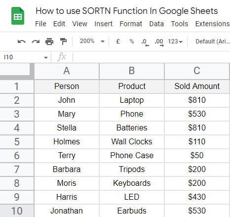
Sample data set
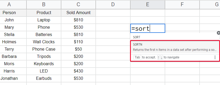
Step 2
Write the SORTN function in a cell where you want to get the result.
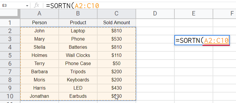
Step 3
Pass the data range as on only argument
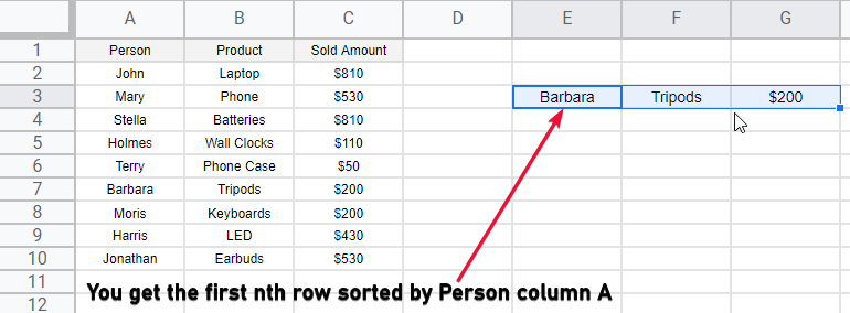
Step 4
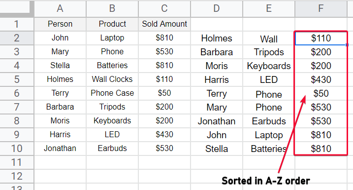
Hit Enter, you can see the first nth row is returned that is sorted first in A-Z order
How to use SORTN Function in Google Sheets – Specifying Number of Rows to be Returned
In this section, we will learn how to use the SORTN function in google Sheets with one parameter to specify the number of rows to be returned in dealt A-Z order. To do this we need to pass one more argument which is the second argument of the SORTN function.
Step 1
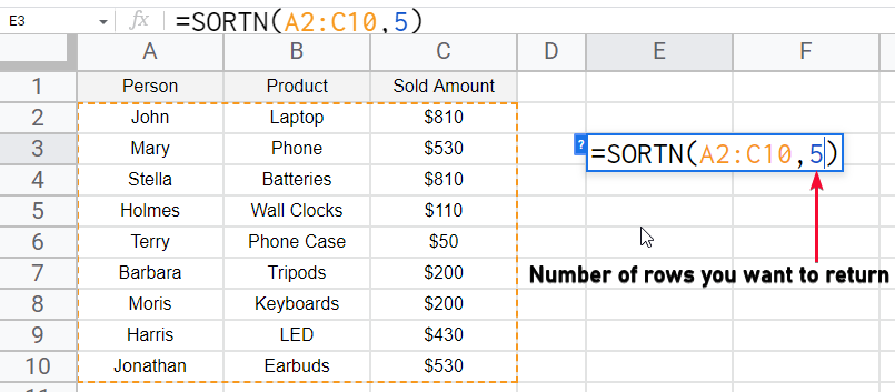
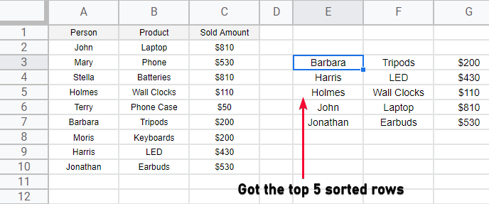
Add the second argument, the number to return the rows (e.g., 3)
Step 2
Hit Enter and the same number of rows will be returned
How to use SORTN Function in Google Sheets – Returning Top 5 – Disregard Ties
You can return the top 5 items from the dataset based on A-Z without any ties rows. The formula will be very simple.
Step 1
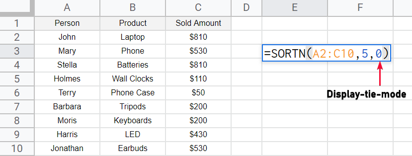
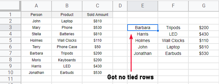
Add 0 as the third argument to specify the 0 ties.
Step 2
Hit Enter and you get the top 5 of your data without any ties
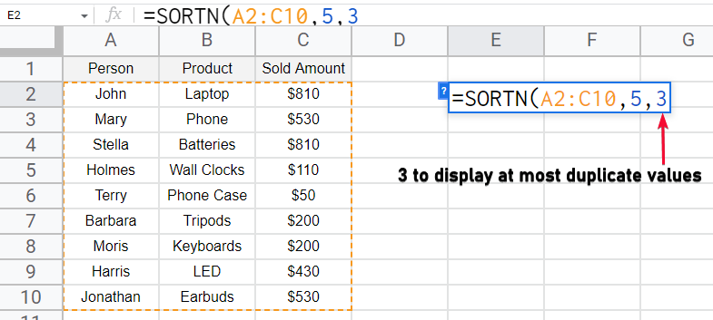
How to use SORTN Function In Google Sheets – Returning Top 5 with tied rows
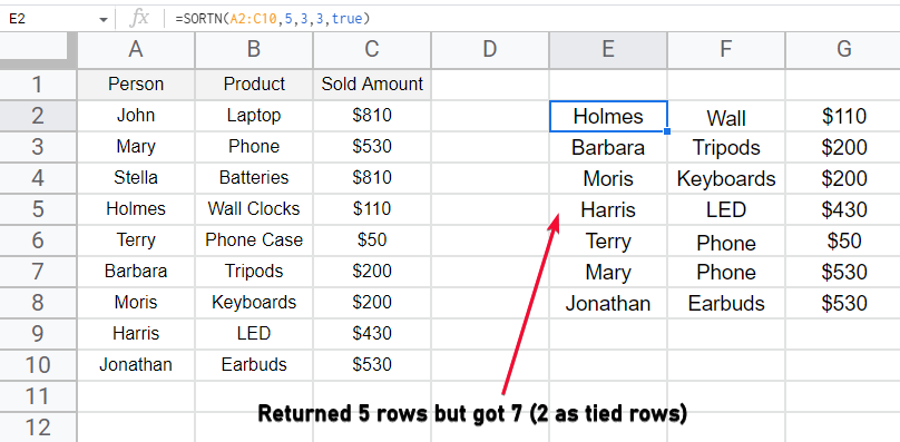
Now tied rows are the rows that have the same value in the column by which we are sorting the data, in this case, we will return the 5 rows but will get more rows if matched with the highest numbers (as if there are some duplicates) if there are no duplicates, we will get only 5 items(rows).
Step 1
Changing the third argument (display-ties-mode), we will specify 3, as we want to show duplicates for each unique row.
Step 2
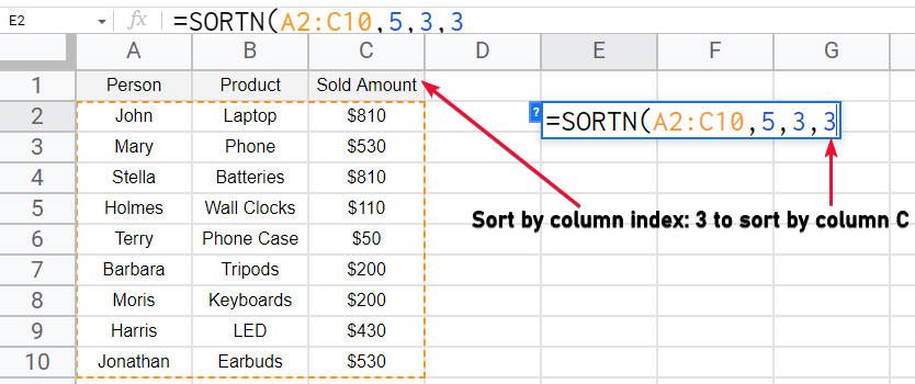
Sort the data using column C (as column C has duplicate values)
Step 3
Hit enter, and you can see more than five rows returned.
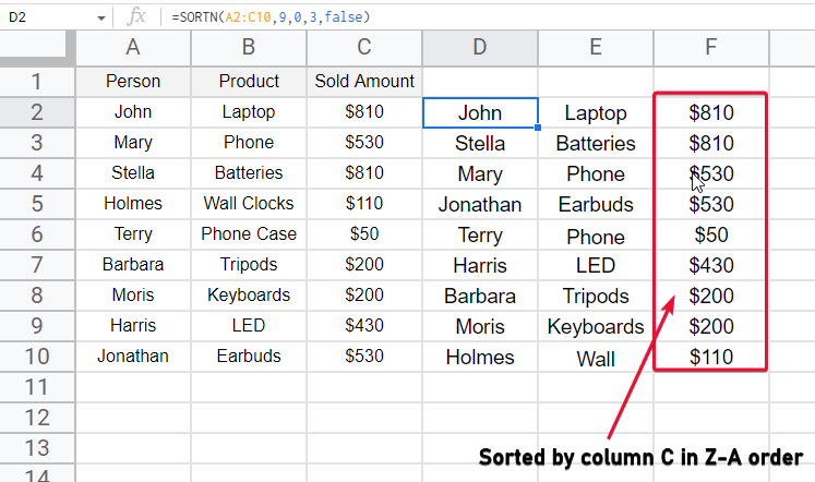
How to use SORTN Function in Google Sheets – Sort By Other Columns
You may need to sort the data by other columns maybe you don’t want to sort the data by names, or by product name, because sorting with them does not make any sense, instead, you may want to sort the data by amount, the sale amount it makes sense the top selling products on top. So, in this section, we will see how to use the SORTN function in google sheets to sort by another column.
Step 1
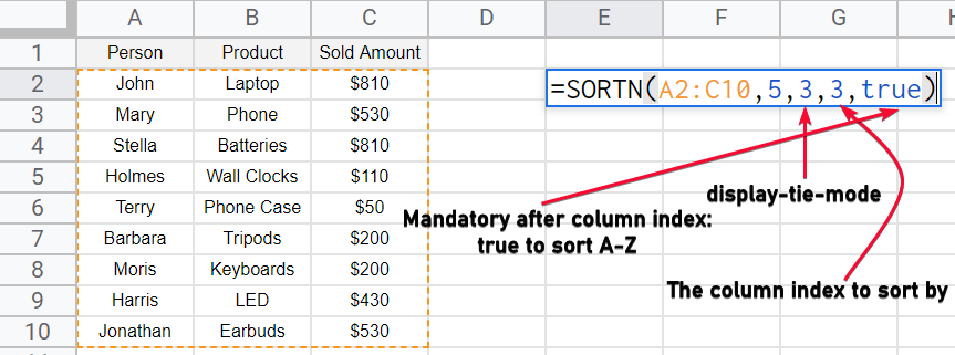
Add the fourth argument as the column index to specify which column to pick to sort by.
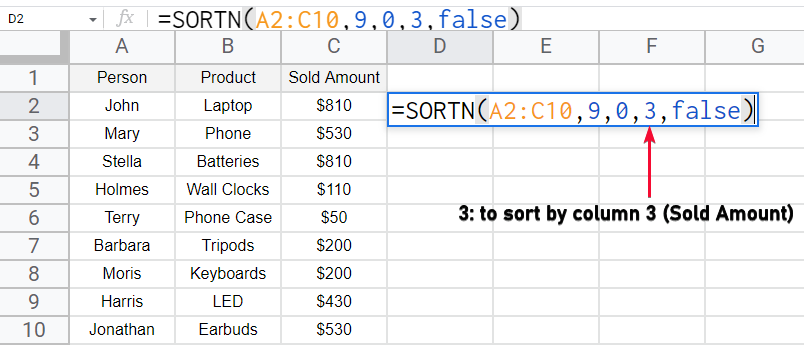
Step 2
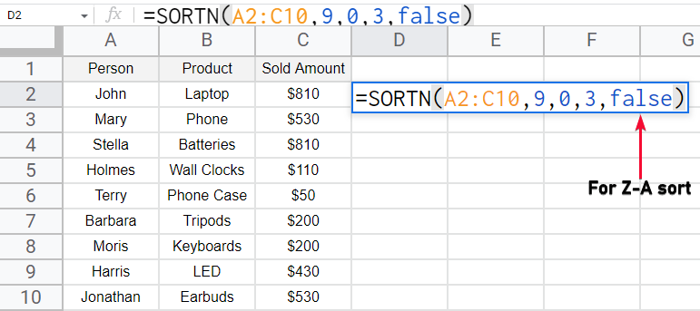
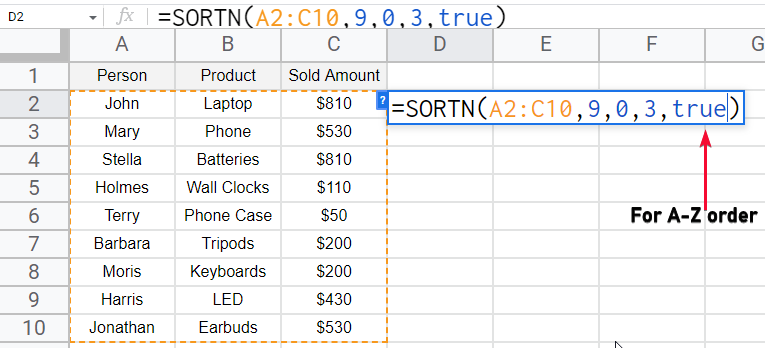
Select next mandatory argument pass true or false or A-Z or Z-A order respectively.
Step 3
Hit enter and your data is now sorted by the specified column
Note: you can also pass a column that is outside of the range you passed in the SORTN function.
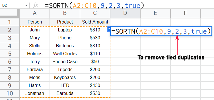
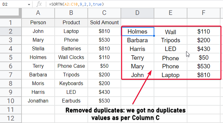
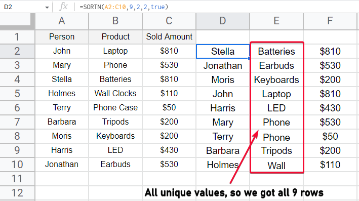
How to use SORTN Function in Google Sheets – Removing Duplicates
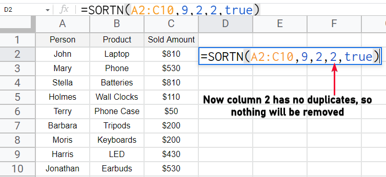
Now in this section, we will see how to get the actual unique range without any duplicate values, for this purpose, we will use the display-ties-mode argument and will change it by 2, which means to Show at most the first nth rows after removing additional or duplicate rows.
Step 1
Changing the third argument, (display-ties-mode), we will specify 2, as we want to at most of the first nth rows after removing duplicate rows.
Step 2
Hit enter and you can see no duplicates are there.
Download/Copy Google Sheets Workbook
Notes
- The range is sorted only by the columns you specify in the formula, the other rows are returned in the same order they are not sorted. They will appear in their original position
- If sort-column1 and is-ascending1 are skipped, the sort will be performed on the lowest-index column in the range (i.e., the first column), with subsequent columns used to sort if there are any ties.
- Most of the arguments are optional, if you don’t use any argument only pass the range you will get the first row in return.
- You can use any other column index out of the selected data range to sort by.
- SORTN expects all the arguments after 3 in pairs.
- If you specify the column index to sort by, then you must need to specify the next argument as well which can be true or false.
Frequently Asked Questions
Can I use the SORTN function to automatically sort my dataset in Google Sheets?
Google Sheets offers the SORTN function for sorting data in google sheets automatically. Whether you want to organize information, arrange rows, or categorize columns, SORTN can help. By specifying the dataset you want to sort and the number of items to display, you can effortlessly rearrange your data. Try SORTN to efficiently manage your Google Sheets.
Conclusion
Wrapping up how to use the SORTN function in google sheets. We have learned various methods and use cases to understand the SORTN function in detail. We have seen how each parameter works, and what are the limitations of the parameters, we have seen optional arguments and also discussed what happens when a parameter is skipped, we discussed default values, and also saw how to perform ascending and descending order sort. I hope you guys have gone through and understood each method, I will recommend you to practice each method and you will never get any problem using SORTN Function in google sheets.
So that’s all from how to use the SORTN function in google sheets, I will see you soon in another tutorial, till then take care of yourself, share with your social friends, and don’t forget to subscribe to us. Thank you, and have a nice day. Keep learning with Office Demy.
