
To Use the IMPORTRANGE Function in Google Sheets
- Select the cell for your imported data.
- Enter “=IMPORTRANGE” and include the source file’s URL, sheet name, and desired data range.
- Press Enter; if an error occurs, grant permission to access.
- The range is imported, and any source data changes will auto-update.
OR
- Select the data range you want to export.
- Under “Data,” choose “Named ranges” and assign a name to the range.
- In your destination file, select the cell for imported data.
- Enter “=IMPORTRANGE” with the source file’s URL and named range.
- Press Enter, and the named range data is imported.
In this article, we will learn how to use IMPORTRANGE Function in Google Sheets.
Now in Google Sheets, we have various ways to connect two individual Google Sheets files and share data within the files or copy some parts. Similarly, we have IMPORTRANGE, an easy function to connect two or more spreadsheets and makes it very quick and easy for us to transfer data among multiple workbooks. Now since it’s a built-in function we need to follow the syntax, below we will see and understand the syntax.
Use Case of IMPORTRANGE Function in Google Sheets
IMPORTRANGE Function is pretty helpful when we have big data and the data is placed in multiple files, if we select a cell in a google sheets file and write the equal sign (=). And then we go to another worksheet and select a range of data from there, the previous file will not collect the cell references of the range we selected. This is because of cross files compatibility, in other software products like excel we can do this, they allow cross files compatibility. But since google sheets completely work on web so they don’t allow such compatibility features without proper reference, so the IMPORTRANGE is the solution google sheets provide us. We will see how to use it and how it works to learn how to import data from other google sheets files and workbooks.
- Data import is very quick and easy
- You can import big data
- Real-time sharing
- Automatically updates data from the source data
How to Use IMPORTRANGE Function in Google Sheets
To learn IMPORTRANGE Function in google sheets we have some methods and some examples using the examples we will see how we can use this function to make our data and range transfer easy within google sheets files and workbooks. Before that, we have to understand some basics about the function.
=IMPORTRANGE(spreadsheet_url, range_string)
- The IMPORTRANGE is the Function name
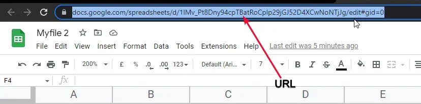
- Spreadsheet_url is the URL (link) of the file from where you want to import the data range
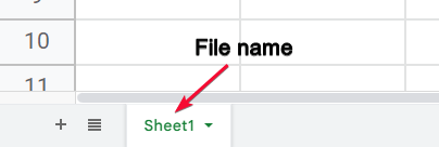
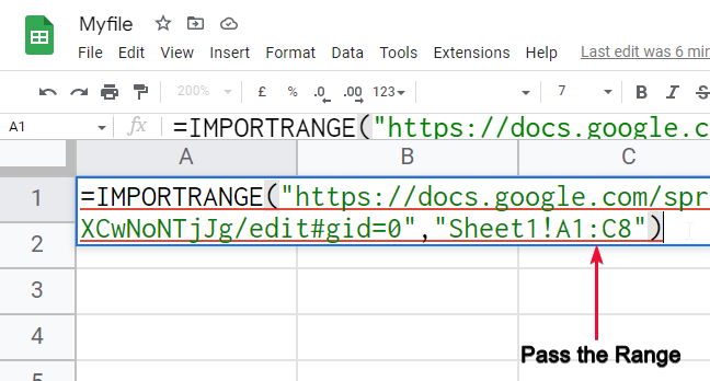
- Range_String is the range of the data (A2:C10), followed by the file name of the workbook if there are multiple files.
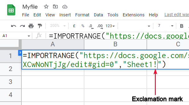
Note that there is a ! mark between the range and the sheet name.
How to Use IMPORTRANGE Function in Google Sheets – To Import a Normal Range
In this section, we will learn how to use IMPORTRANGE Function in Google sheets to import a normal range from another workbook. In this section, we have multiple google sheets files and we will learn how to import data from each file to another file.
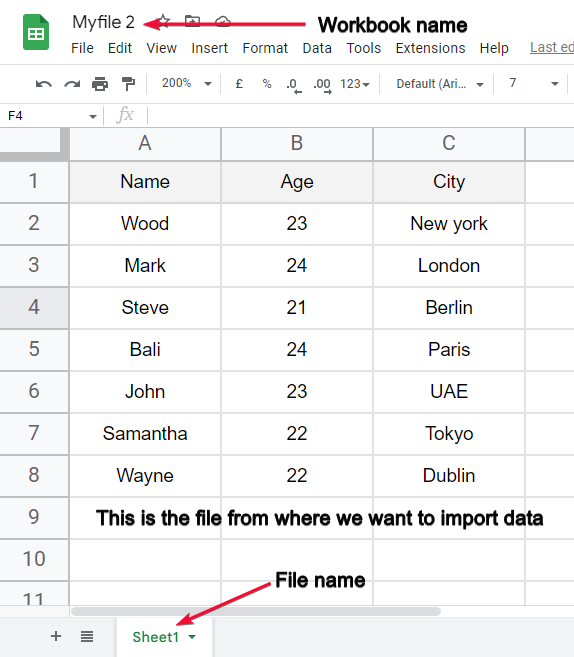
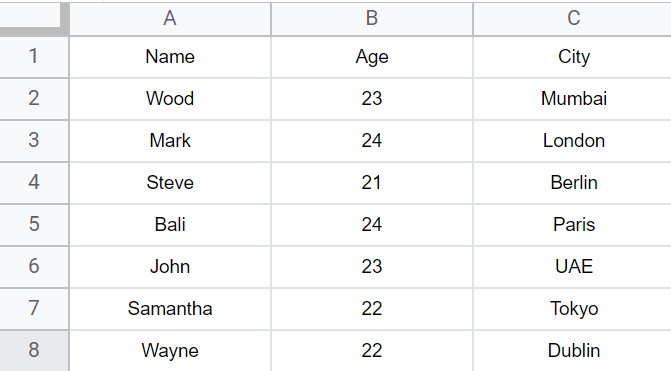
So, I have two files 1 is empty and the other has some data, I will fetch the data in the empty file
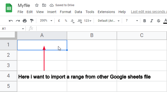
Step 1
In the google sheets file, click on the cell where you want to import the range
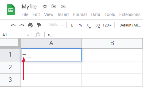
Step 2
= sign
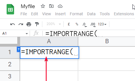
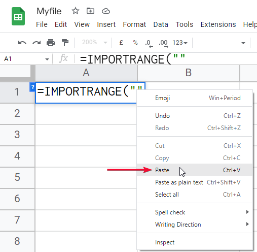
Step 3
IMPORTRANGE Function
Step 4
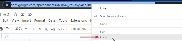
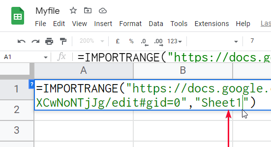
Pass the URL or spreadsheet id inside double quotes
Step 5
Pass the file name
Step 6
Exclamation mark “!” after the file name
Step 7
Pass the data range (i.e., A2:C10)
Step 8
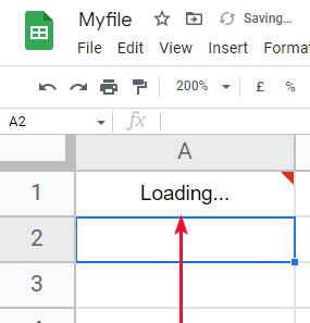
Hit Enter, you may see an error
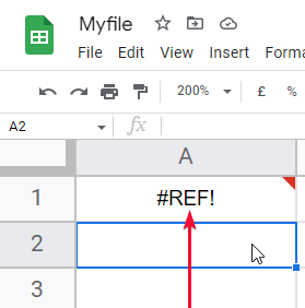
Step 9
Understanding the error
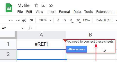
Step 10
Resolving the error by allowing access
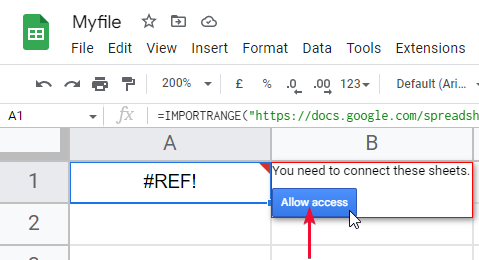
Step 11
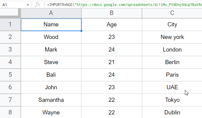
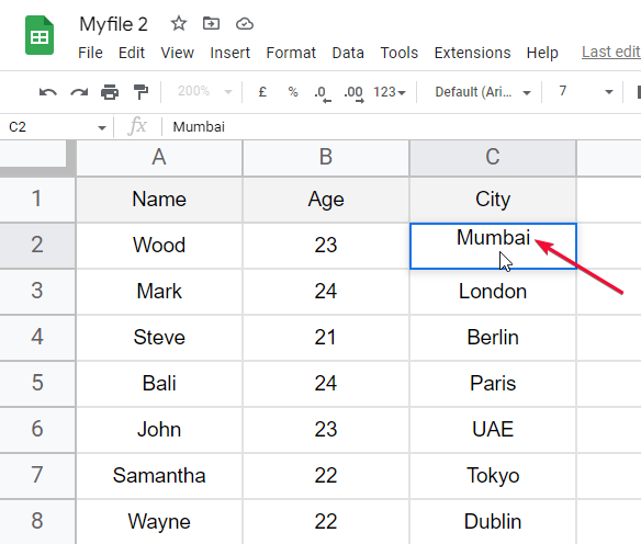
Success, the range is imported accurately
Step 12
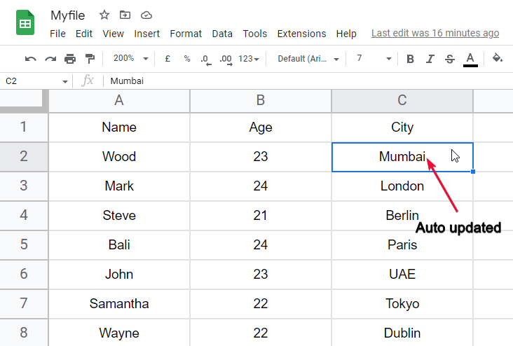
Make some changes in the source data
Step 13
You can see the change is automatically updated.
This is how simply you can work on IMPORTRANGE Function and import your ranges and data from one google sheets file to another.
How to Use IMPORTRANGE Function in Google Sheets – Using Named Range
Named range is nothing but a concept to name our data ranges. This is exclusively available in google sheets and it’s pretty useful we all get confused and can’t remember the range names so this is the ultimate solution. We will mark the ranges we want to import in a sheet, then we will convert those ranges to named ranges, we will assign good names to all ranges and it will make it easier for us to call that range from the name instead of actual cell range.
Many times, we need to have a lot of data to import from various sources and we are confused with the ranges, the column and row names, of course, we cannot memorize all the data ranges, so there is a solution to this problem. Whenever you need to have a lot of import data from multiple spreadsheets file you need to learn this technique to save your time and energy
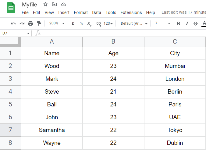
We have some datasheets from which will collect data ranges and will import them into the final file.
Step 1
You need to have multiple workbooks or google sheets files to follow me with this example
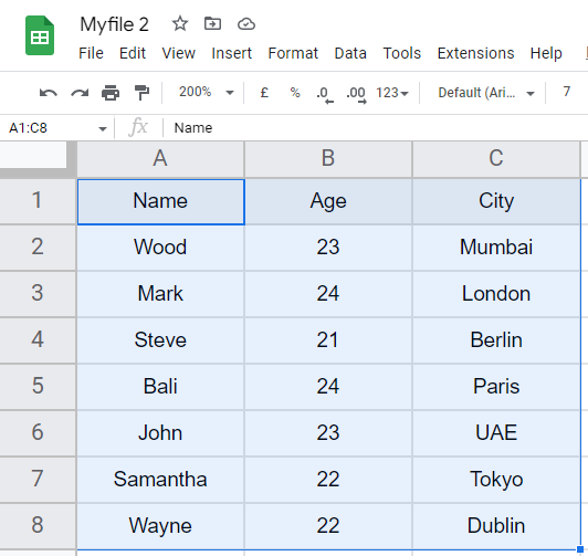
Step 2
Select the range of the data you want to export into the final sheet
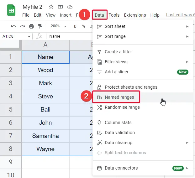
Step 3
Go to Data > Named Ranges
Step 4
Give a name to the selected date range
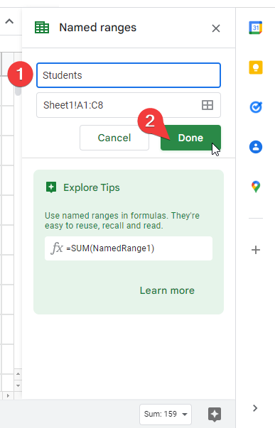
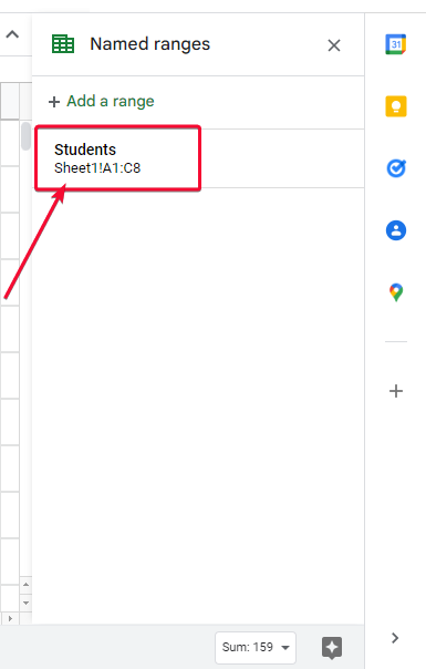
Step 5
Click on done, and your range has got the name
Step 6
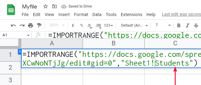
Now using IMPORTRANGE Function similarly to import this range, but this time we will use the range name, not the cell references.
Step 7
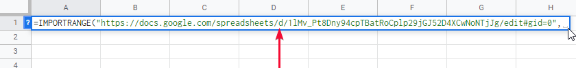
The overall syntax will be like below
=IMPORTRANGE(“https://docs.google.com/spreadsheets/d/1lMv_Pt8Dny94cpTBatRoCplp29jGJ52D4XCwNoNTjJg/edit#gid=0″,”Sheet1!Students”)
Step 8
Press Enter, you can see we have got the same result
Tip:
Know that when you use IMPORTRANGE Function for the very first time on your sheet, after completing the function parsing the values, and when calculating the answer, it will return a reference error. Don’t worry about it, you have not done anything wrong it is the natural behavior of google sheets. This is an importing function and this error is only a warning (read the error message), it’s a permission, google sheet’s asking you to allow to access the data from other sources (workbooks or google sheets files), when you allow it, google sheets has got the knowledge that you (as a google account holder) authorize this spreadsheet and now google sheets will link that sheet with your current sheet. This is the entire process.
Notes
- Use Named ranges when you have multiple ranges to import from one or multiple sheets or workbooks.
- Named ranges are easy to deal with
- The function returns an error on the first-time users, it’s a warning simply give the permission to allow it to access the data from other sheets, files, or workbooks one time then it will never ask for it again for the same data sheets.
- IMPORTRANGE is an importing function, it helps us import the data from other google sheets files directly with live updates
- Remember that importrange does not copy formatting or style, it only copies values or formula-driven values.
- Importrange can work on the URL, and also on the key, a spreadsheet key can be used instead of the entire link and it works perfectly.
FAQs
Why I am facing a reference error when importing a range?
Yes, for the first time the IMPORTANCE function will give you a reference error, read the error and it will ask for permission to import the range from the sheet you have specified by providing the URL and range. This is for the security and safety purposes of data, once you have to permit by clicking on allow button and then it will give you the range imported from that sheet or workbooks, next time you will use the IMPORTRAGE function then it will not ask for any permission and no error will be thrown. This is one-time authentication and after allowing it’s allowed for a lifetime.
Can I use Named Ranges for other purposes?
Named ranges is a new concept introduced by google sheets for naming several ranges in a big data set for better identification and minimizing the reference error and also the problem of memorizing the ranges every time using in a formula. For other purposes, surely yes. Named ranges are not associated with IMPORTRANGE or any other function exclusively. Named Ranges are independent and can be used in any condition, you can use them without using any other formula or function, you can use them directly just to rename the important ranges or the ranges that you think will be used in the formula or function frequently. The main purpose of the named range is to rename the range of cells, logically it can be applied even on a singular cell.
Conclusion
So here, I hope you have gone through the entire tutorial and have learned How to Use IMPORTRANGE Function in Google Sheets. I have covered the basic function and we talked about the syntax as well, then we moved on to the method and we learned step by step how to use IMPORTRANGE Function in google sheets. We talked about the error that is a first-time error for the permission, we have also seen the auto update of data on any change made on the exporter files. We have seen the change is automatically updated in the file, then we moved on and learned a technique called Named ranges exclusively available in google sheets, we have seen how Named ranges work and how we can use them, and how they help us while importing the data. We did an example using Named ranges inside the IMPORTRANGE Function.
So, that’s all for today’s tutorial I hope you have now learned how to use IMPORTRANGE Function in google sheets, see u soon with another tutorial till then take care. Share this article with your friends and don’t forget to subscribe Office Demy blog. Thank you have a nice day.
