How to Make an Inventory List on Google Sheets

Hi, today we will learn how to make an inventory list on Google Sheets. Stock Maintaining and keeping records for items and orders is always a big challenge for a storekeeper. Then hiring a professional to make an inventory list can be very costly as well. Then why don’t we make an inventory list for our store ourselves? Yes! Office Demy has brought a tutorial below on how to make an inventory list on Google Sheets so wait for what, let’s get started.

Is it better to Make an Inventory List on Google Sheets?

If you want a free inventory list, then I must say that Google Sheets is the best choice because it’s a free web-based software and provides enough tools to make a professional inventory list. Google Sheets does not only make a creative inventory list but also makes it automated through which you can easily monitor your inventory and keep updated by stock.

Let me show you practically with the help of the following demo.

How to Make an Inventory List on Google Sheets?

There is no technical method to make an inventory list in Google Sheets but a need for logical expressions. Firstly, it’s up to you what you want to include in your inventory list. In the following tutorial, I will describe to you enough different factors through which you can make an effective inventory list for yourself in Google Sheets.

Step 1

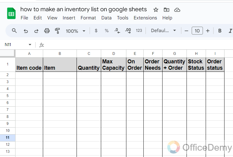
Firstly, create a structure of an inventory list in Google Sheets and add headings whatever you want to include in your inventory as I have made the following columns.

Step 2

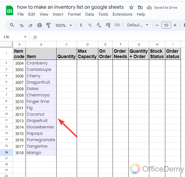
In my inventory list, the first two columns are for Item Names and their codes, so here first we will add items with their codes according to my store data.

Step 3

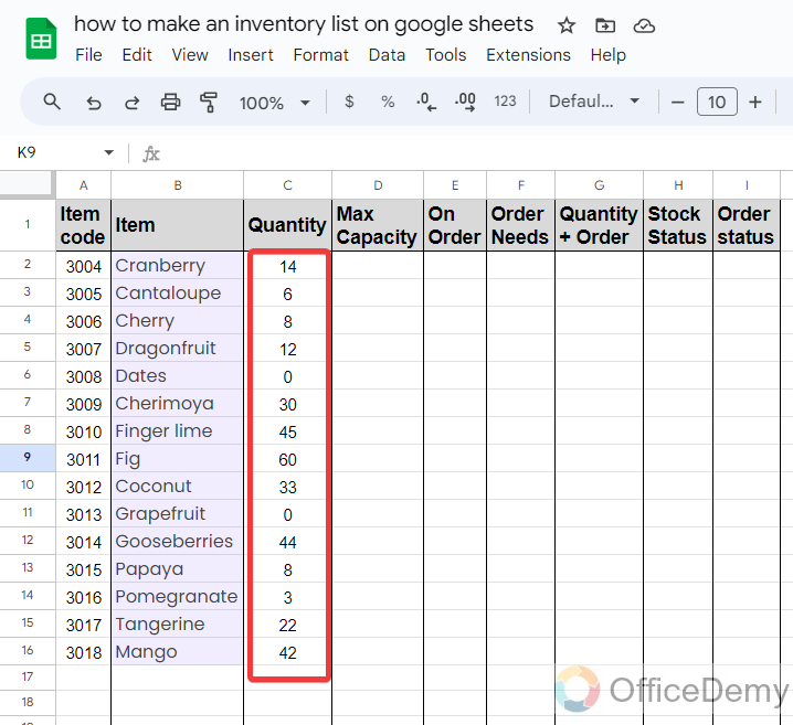
After writing the names of the items, I will add here the quantity of the products that you will have to type manually by checking your stock remaining.

Step 4

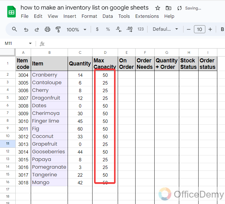
In the next column, I have mentioned the maximum capacity of the products that my store can stock to make several calculations later. These values will be fixed once you have written.

Step 5

Now, in my inventory list, there is a column for “Order’s Needs” where Google Sheets will tell us, how many quantities of product are needed to order by calculating the record.

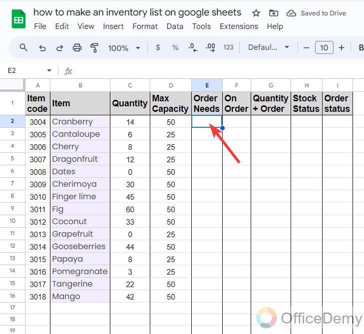
Step 6

In this column, I can get the value by just subtracting the max quantity from the actual quality of products, but if the actual quantity reaches above the max capacity, then it goes negative values so here, I will use the “Max” formula where first criteria will be “Max capacity” subtract from the “Actual quantity” as can be seen in the following picture.

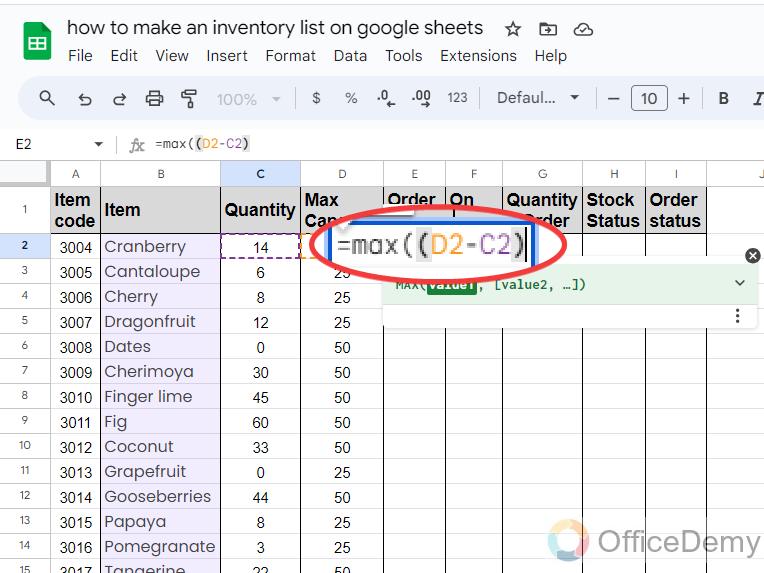
Step 7

After giving the first, the second max criteria will be the “0” as mentioned below. This will calculate the needed quantity of the products, if there is no need then it will show the value zero.

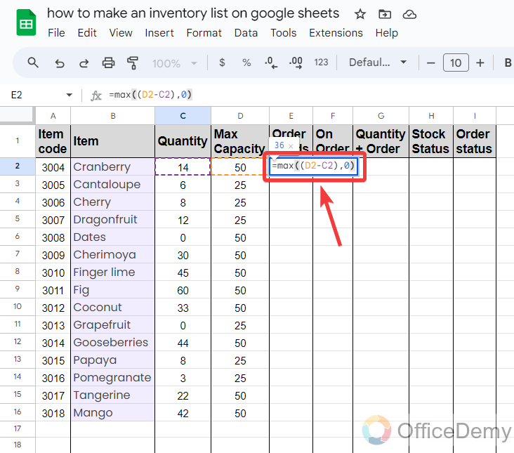
Step 8

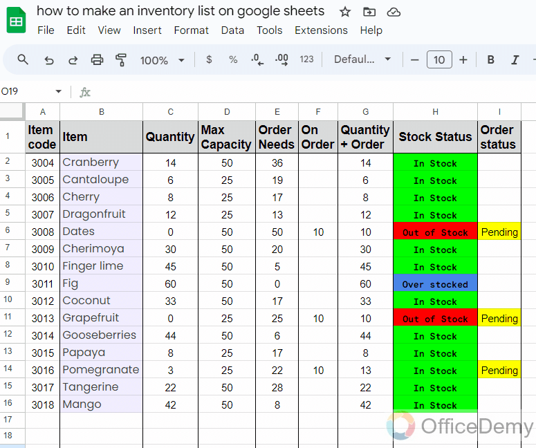
Once you have completed writing the syntax press the Enter key to get the result. As you can see in the following picture, we have just 14 cranberries out of 50, so we need 36 as shown below.

Let’s drag the formula on other cells.

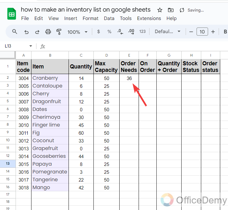
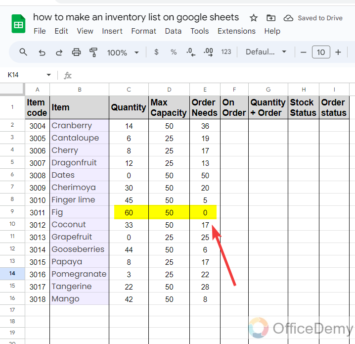
Step 9

We have got all the results as can be seen below, if you observe row number 9, the quantity of fig is overstocked so the “Order Needs” returns to the “0” instead of the negative value.

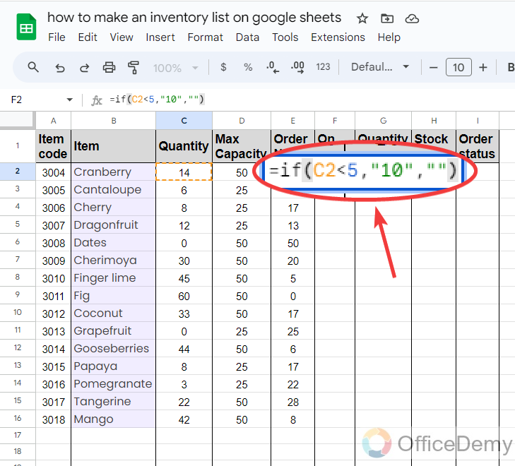
Step 10

This column may be additional or may change according to your preference, Here I have specified the criteria by the “IF” function. If the quantity reaches its lower about less than 5 orders minimum of 10 items otherwise leave a blank cell. As you can see the pattern of the syntax is in the following screenshot.

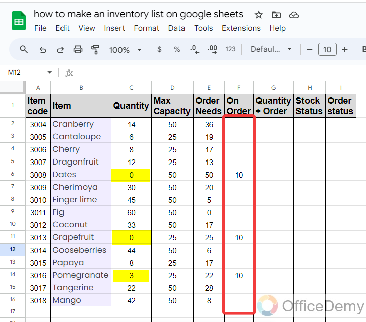
Step 11

Here is the result for this column, as you can see if the quantity of items is less than 5 it has orders 10 more automatically. It was my opinion you may skip it or increase the number of orders as you desire.

Step 12

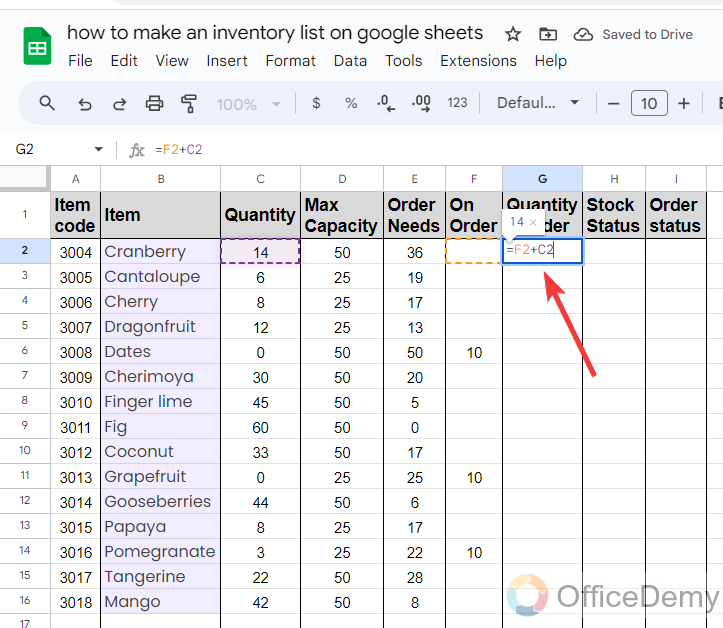
If there is an order is placed for any item in your inventory list and you want to look at how many items will be in stock after the order reaches, then you can monitor from the following column “Order + Quantity” where I have inserted only simply sum formula to sum order items and quantity as shown below.

Step 13

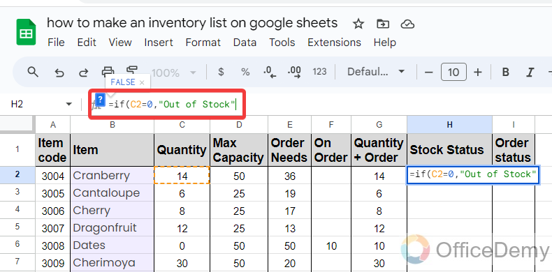
Then the next column in our inventory list is for Stock status, in this column we will apply three different conditions with the “IF” function. Here, you can see the first condition, “=IF (C2=0″, “Out of Stock” that means if the quantity reaches zero then it will show “Out of stock” in the cell.

Step 14

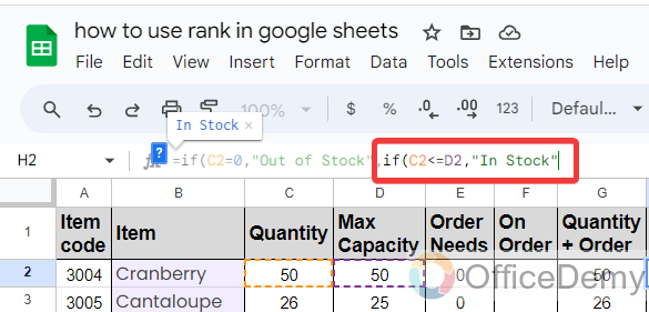
In the same way, in the second condition, I have given the criteria that IF C2<=D2, “In Stock” that means if the actual quantity of items will be less than or equal to max capacity, display it as in stock.

Step 15

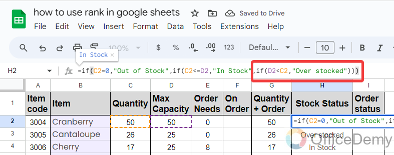
For the third condition, I have written the syntax IF D2<C2 means if stock reaches above the max capacity, then show it as “Overstocked” as highlighted in the following picture.

Step 16

The result will be as follows when we press the Enter key, as you can see where the Stock is zero it is showing Out of Stock, where the stock is above the max capacity it is displaying Over stock and rest are the In stock.

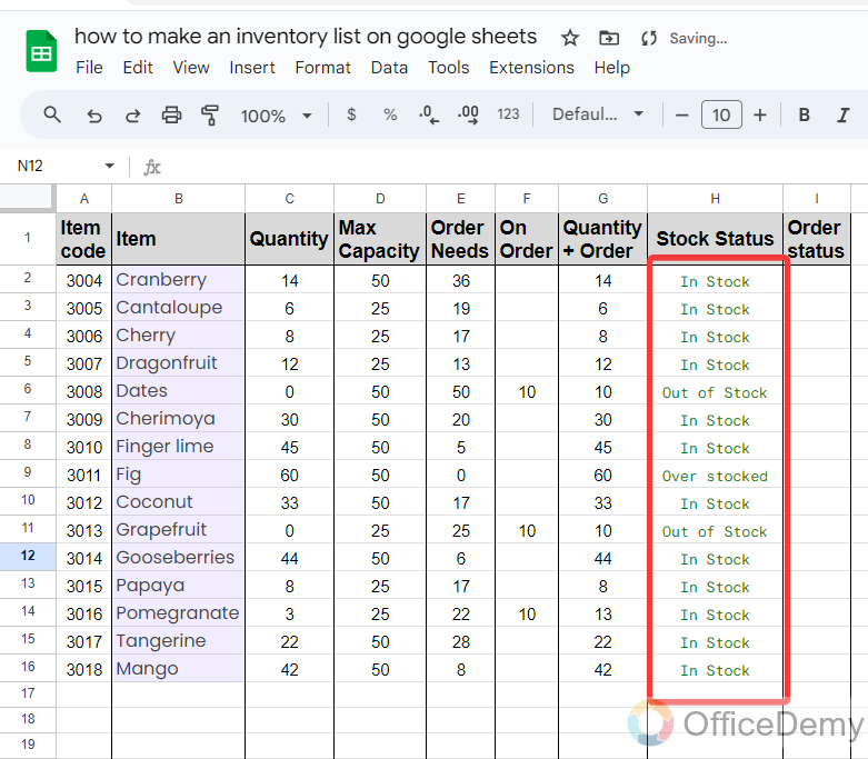
In this way, we can easily monitor which items are in stock, out of stock, and overstocked.

Step 17

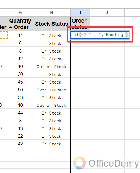
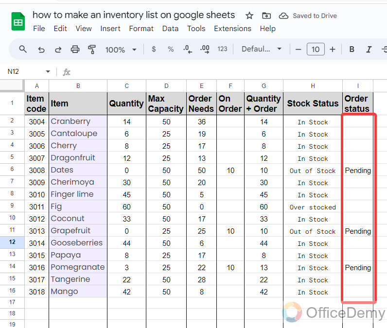
When we order something, we should know whether it has been delivered to our store or not. For that, I have added a column in my inventory list where I have the following formula If(F2=” “,” “, “Pending”),

Where F2 is the value of on-order items. If there’s nothing in order then it will remain empty as well but if we put any item on order in our inventory list, It will automatically display it as Pending in status.

Step 18

As you can see from the result in the following picture, when is order is placed in our inventory list, the order status is “Pending” through which we may know which orders are Pending.

Step 19

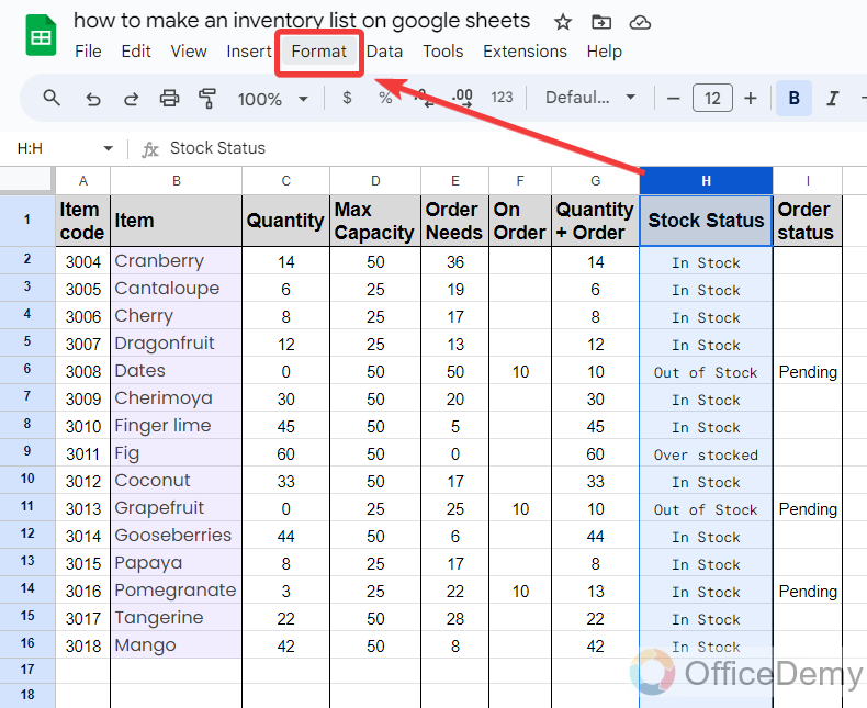
To make a more attractive and creative inventory list I am going to apply some conditional formatting. To apply conditional formatting on the cells, first select the cells then go into the “Format” tab from the menu bar.

Step 20

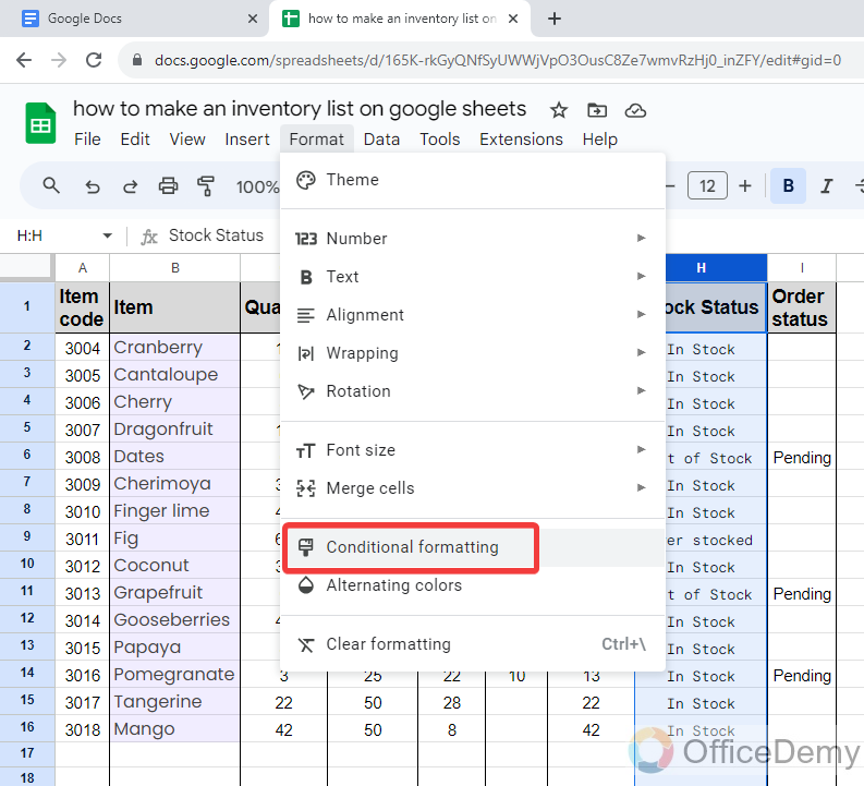
When you click on the “Format” tab, a drop-down menu will open, click on “Conditional formatting” from this menu.

Step 21

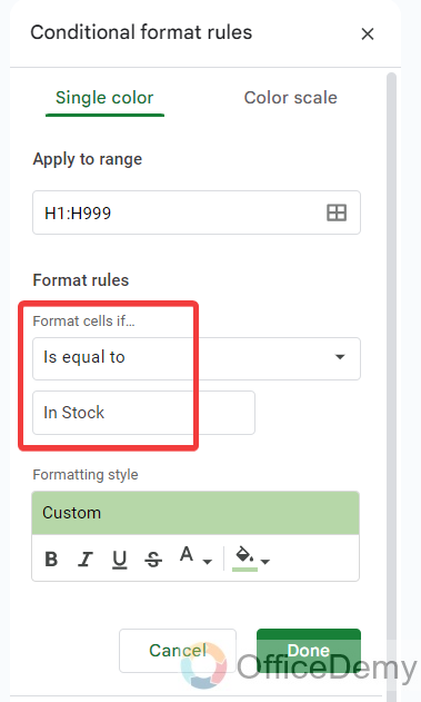
In the stock status column, I am applying a rule that If the cell is equal to “In stock“, fill it with a green color.

Step 22

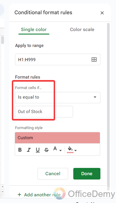
Similarly, for the values of Out of Stock, I have chosen the red color.

Step 23

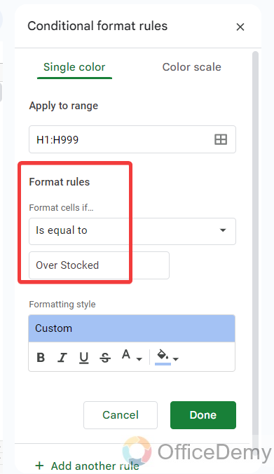
If the cell is equal to “Overstocked” then fill it with a blue color as highlighted below. Once you have applied all the rules click on the “Done” button.

Step 24

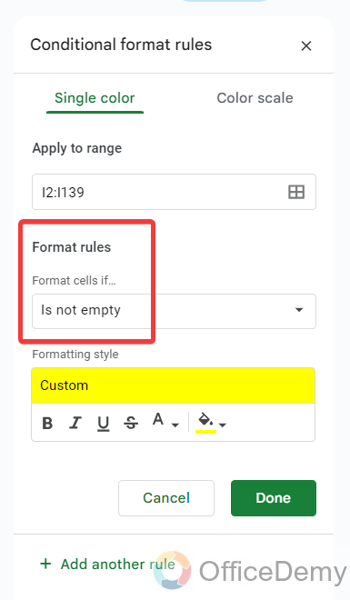
Here, I am also applying formatting in the “Order status” column. If the cell is not empty, then fill it with the “Yellow” color. In this condition, it will highlight the cell as yellow, when it would be “Pending“.

Step 25

It is all done from my side, I have included so many things to make an effective inventory list in Google Sheets as you can see in the following animation showing how perfectly all functions and formatting are working.

Conclusion

Hope the provided knowledge on how to make an inventory list on Google Sheets will scale up your business and your professionalism. If you like the above tutorial, share it with your friends and keep connected with Office Demy.