How to Create a Checklist Template in Google Sheets

Today we are here with the topic of how to create a checklist template in Google Sheets, you can get an idea on creating a checklist template in Google Sheets. Creating a checklist template in Google Sheets is very straightforward as it has built-in options regarding checklists. In this guide I will give you the way to create a checklist template then you can create your own checklist template for any purpose in Google Sheets.

Benefits of a Checklist Template in Google Sheet

Checklists can be very useful in Google Sheets like project management checklists, onboarding checklists, grocery checklists, cleaning baggage checklists, bucket checklists, To-do checklists, etc. These templates are very common and very useful. You may need to make a checklist template in Google Sheets. If you also want to create a checklist template in Google Sheets that is for free, then follow the following instructions.

How to Create a Checklist Template in Google Sheets

The procedure of creating a checklist template in Google Sheets is very fine and easy as Google Sheets has built-in options to insert a checkbox into sheets and also has features of applying Conditional formatting through which you can create an effective checklist template in Google Sheets of any category.

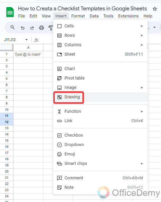
Step 1

Here we are going to create a “To-do list” to make a checklist template in Google Sheets so here first we will add the title of our template. To make a title in Google Sheets we will use the “Drawing” tool of Google Sheets.

Step 2

To make a title, you can use “Word art” or “Text box” but here I am using a shape for creating a title for a checklist template.

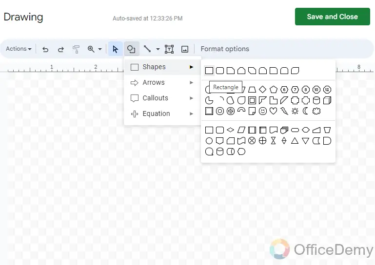
Step 3

Create a shape and fill it with the desired color. To add text in the shape, double click on the shape and write the text as I have written “To-do list” in the following example. You can also format the text with the help of a drawing tool.

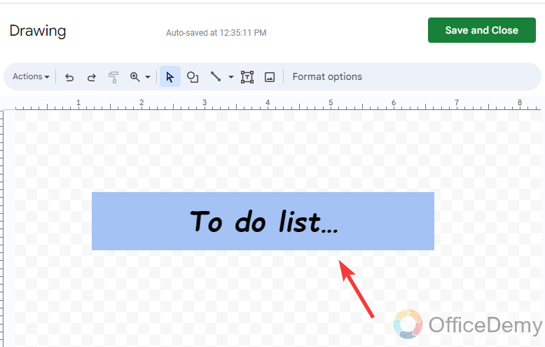
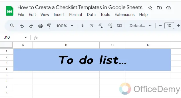
Step 4

To insert your shape into your sheet, click on the “Save and close” button, your shape will be inserted into your sheet as can be seen in the following picture.

Step 5

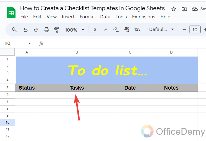
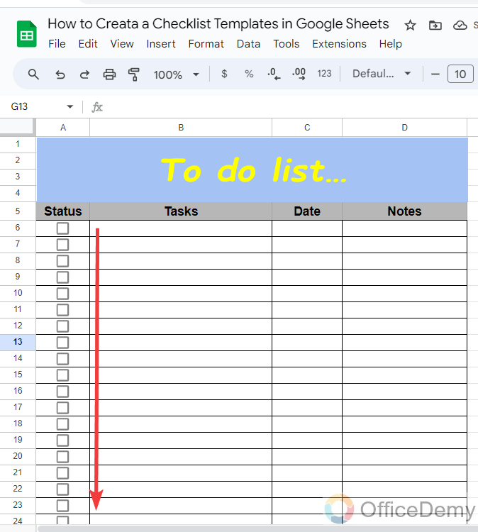
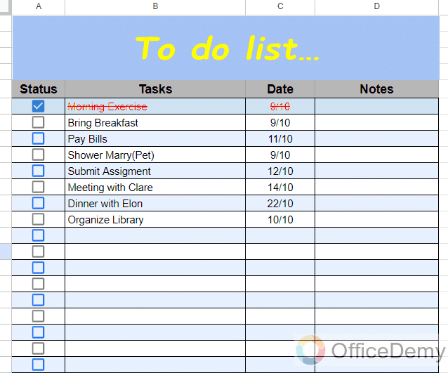
After adding the title for the checklist, we will add headings that we want to include in our checklist template as I have included status, tasks, date, and notes in the following to-do list.

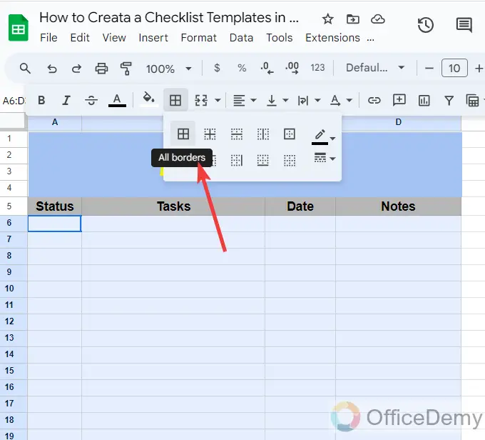
Step 6

After adding the headings, Select the cells that you need in your checklist template to make a to-do list. After selecting the cell border all the cells from the “Border cells” option as directed in the toolbar of Google Sheets.

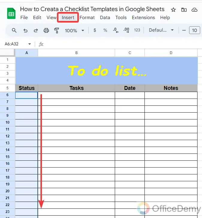
Step 7

As we are creating a checklist we will have to add checkboxes in the template that we will insert in the column of Status. To insert checkboxes first select all the cells as I have selected below.

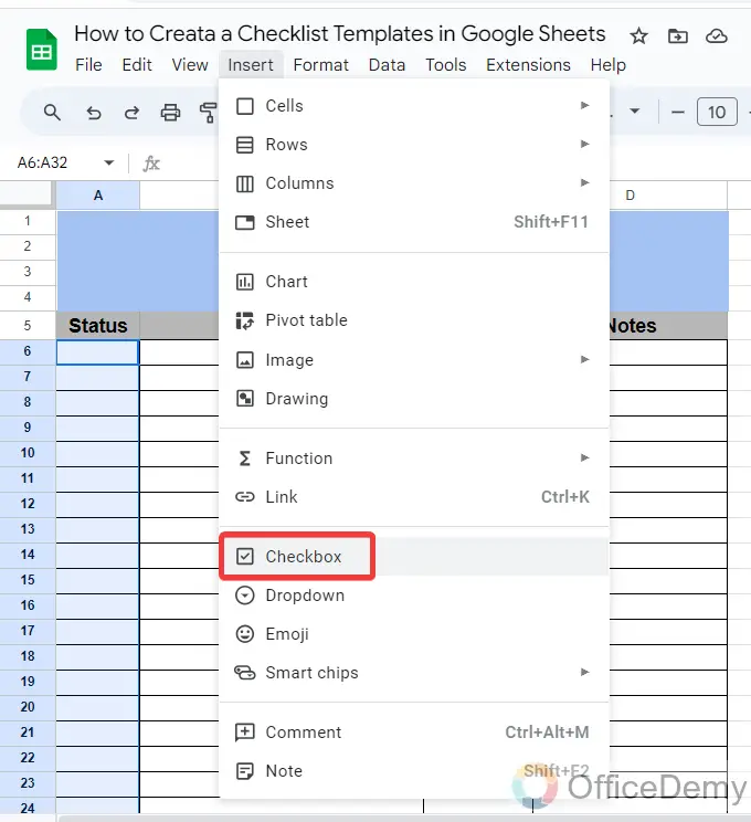
Step 8

After selecting the cells, go into the “Insert” tab from the menu bar of Google Sheets where you will find the “Checkbox” option as highlighted in the following picture.

Step 9

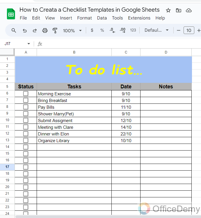
As you click on the “Checkbox” option, checkboxes will be inserted automatically in the selected cell as can be seen in the following picture.

Step 10

After adding checkboxes, write down the Tasks that you want to add your to do list as I have written several tasks in the following example. You can also include dates regarding tasks in your template.

Step 11

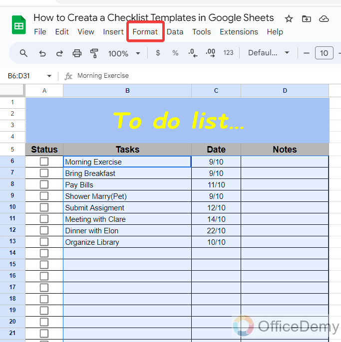
To make your checklist template more professional, we will apply some formatting. To apply any kind of formatting first we will select all the ranges and then click on the “Format” tab from the menu bar as highlighted below.

Step 12

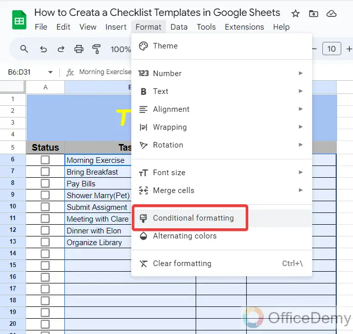
When you click on the “Format” tab from the menu bar, a drop-down menu will open where you will find “Conditional Formatting” as highlighted below.

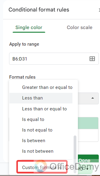
Step 13

Clicking on the “Conditional formatting” option will give you a pane menu on the right side of the window where you can apply formatting. On this pane menu select the “Format rule” to “Custom formula” as highlighted below.

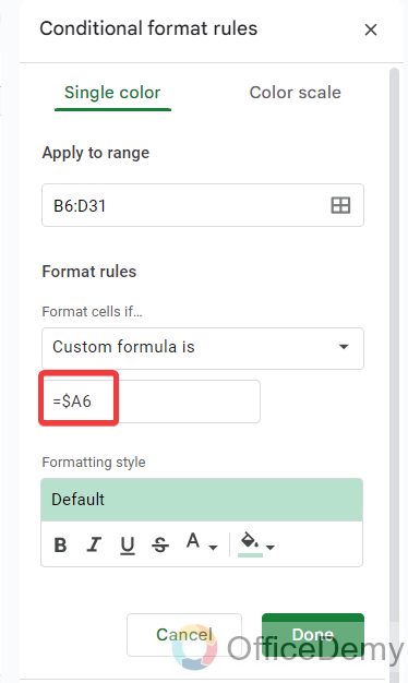
Step 14

In the custom formula, we will write the formula “=$A6” which will indicate when we mark the checkbox in the template and format the cell.

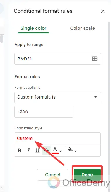
Step 15

After adding the formula, set the formatting that you want to make in your template, as here I am applying the “Strikethrough” on the text and formatting the text with red color as can be seen in the sample below. Click on the “Done” button to save these formats.

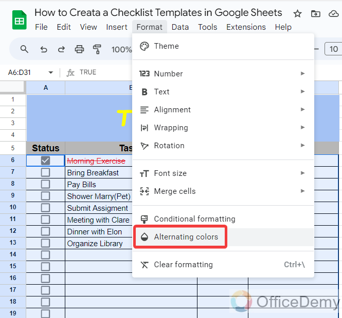
Step 16

We have almost finished creating a checklist template in Google Sheets, but here we are also including “Alternating colors” to make our template more attractive. It is optional if you don’t want to add then you can skip it as well.

Step 17

Our checklist template is ready now, as you can see the result in the following GIF image. As you mark the checkbox for any task it will automatically turn red, and a strikethrough will apply to it to mark it has completed the task.

In this simple way, you can create any style & any purpose checklist template in Google Sheets.

Frequently Asked Questions

How to add a progress bar in the checklist template in Google Sheets?

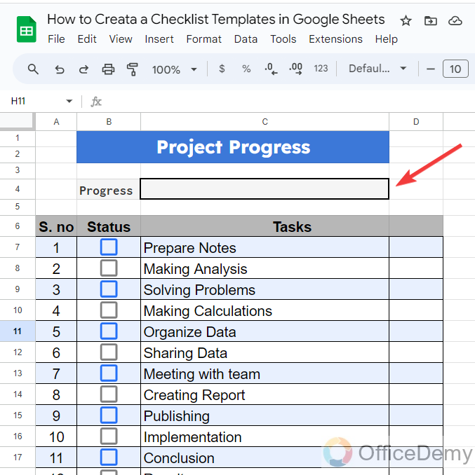
Let’s suppose you are working on a project that contains multiple tasks for which you have created a checklist template for yourself. Now you want to add a progress bar in your checklist to identify how much progress you have made in your project. Then, you do not need to worry about it. You can add an automatic progress bar with the help of Google Sheets functions to make your checklist more progressive.

Step 1

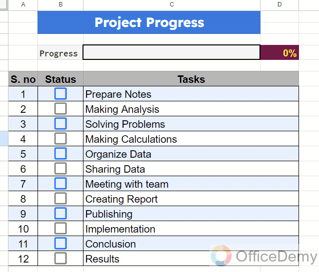
As you can see in the following picture, we have a progress bar in the following checklist template. Let’s see how we can make it functional according to the progress.

Step 2

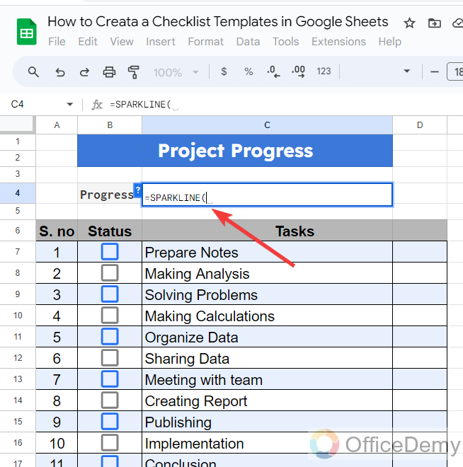
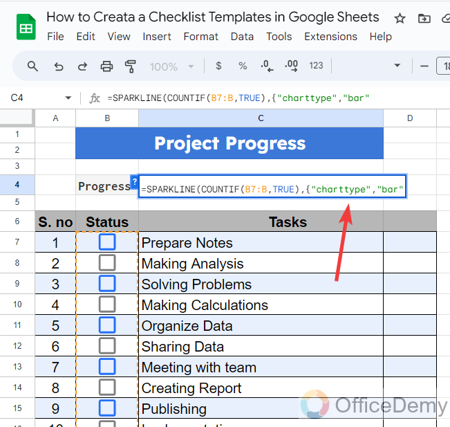
To create a progress bar in the checklist template, we will use the “SPARKLINE” function of Google Sheets. Simply, write the “SPARKLINE” with an equal sign in the progress bar cell as directed below.

Step 3

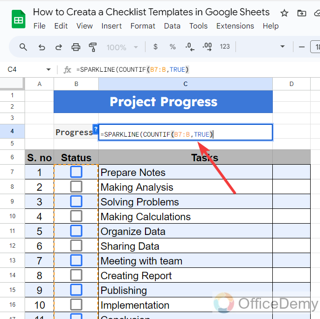
After the SPARKLINE function, I will add the “COUNTIF” function of Google Sheets, to count marked checks in the list. After starting the CountIf function, we will write the range of checkbox columns as written in the following picture.

Step 4

After completing the “COUNTIF” function, let’s complete the “SPARKLINE” function first we will specify the Chart type as I have specified the “Bar” to make a progress bar.

Step 5

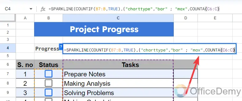
According to the Sparkline function, we will provide the max and min range of the Sparkline, by default min range is zero so here we will only describe the maximum range which is the range of all tasks in the checklist.

Step 6

In the last part of the syntax, we will specify the color of the progress bar in the syntax, to specify the color of the progress bar in the Sparkline function first we will write “Color1” and then specify the desired color in quotation marks as I have described “Green” color in the following syntax.

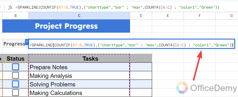
Note: Arguments of the Sparkline function will be in the curly brackets and each argument will be divided by semicolon.

Step 7

If you want to display the percentage of the progress in the following progress bar, then you can also display the progress in percentage with the help of the following formula.

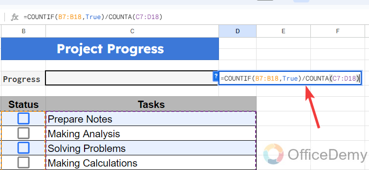
Formula: =COUNTIF(B7:B18,True)/COUNTA(C7:D18)

Step 8

You are almost done by creating an automatic progress bar and progress percentage as well and you can see the result in the following demo.

Do you want to get this Template?

Get a Free “View only” Template here, Go to File > Make a Copy, and use it as per your needs.

Free Checklist Template – Office Demy

Conclusion

A checklist plays a very important role in organizing your tasks, keeping track of things, and mapping out your schedule. Therefore, the above article on how to create a checklist template in Google Sheets is going to be beneficial for you.