How To Use RANDBETWEEN Function in Google Sheets

Today we will learn how to use the RANDBETWEEN function in Google Sheets. The RANDBETWEEN function is a powerful feature of Google Sheets that allows you to generate random numbers within a specified range. In this article on how to use the RANDBETWEEN function in Google Sheets, we will convey a complete guide on using the RANDBETWEEN function in Google Sheets.

Benefits of using RANDBETWEEN Function in Google Sheets

Commonly, when we generate a random number in Google Sheets, it gives us only the numbers between 0 and 1. The most beneficial advantage of the RANDBETWEEN function is that you can find a random number between the specific values that you want to find with the help of the RANDBETWEEN function.

Moreover, you can also RANDBETWEEN function with other functions to select a string randomly in Google Sheets. Let’s see how to use the RANDBETWEEN function in Google Sheets.

How to Use RANDBETWEEN Function in Google Sheets

In this article, we will discuss several examples of using the RANDBETWEEN function and then will also discuss the usage of RANDBETWEEN with other functions.

1. RANDBETWEEN function examples
2. RANDBETWEEN function with INDEX function
3. RANDBETWEEN function with CHOOSE function

1. RANDBETWEEN Function Examples

In this section of the tutorial, we will discuss some different examples of using the RANDBETWEEN function of Google Sheets. Let’s look at some examples of how the RANDBETWEEN formula can be used in Google Sheets.

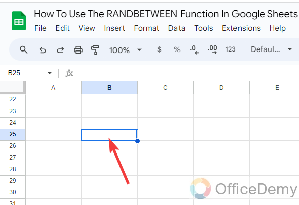
Step 1

First of all, select the cell and place your cursor where you want to use the RANDBETWEEN function in Google Sheets as I have selected in the following picture.

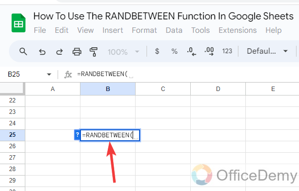
Step 2

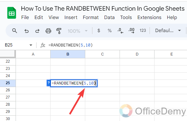
After selecting the cell, start writing the “RANDBETWEEN” with an equal sign to start the RANDBETWEEN function.

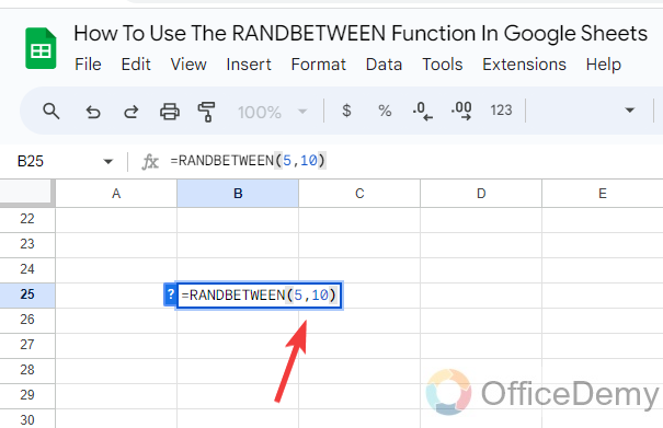
Step 3

After starting the RANDBETWEEN function, we will write the arguments of the function as the RANDBETWEEN function searches the random numbers between only the two values so here we will write only these two arguments that is lower limit and upper limit.

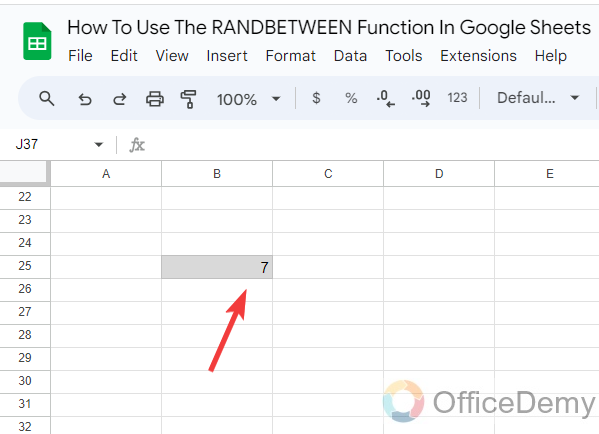
Step 4

Once you have completed the formula, press the Enter key, and you will get the result in a random number between the specified value as resultant below.

Step 5

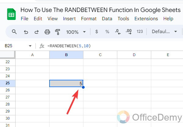
You will get different results every time you enter these values. Let’s check by finding the random number between “1,10” again and see what value we get this time.

Step 6

As you can see the result in the following picture shows that we have gotten the result “5” but previously we found “7“. Similarly, if you find it again it may give you a different random number.

Step 7

If you want to find a random number between two negative values, then you can also find it by the RANDBETWEEN function, but you must be careful about putting the correct order of the values. First, we will have to set the lower limit and then the upper limit. In the following example we see “-50” is the lower limit and “-30” is the upper limit.

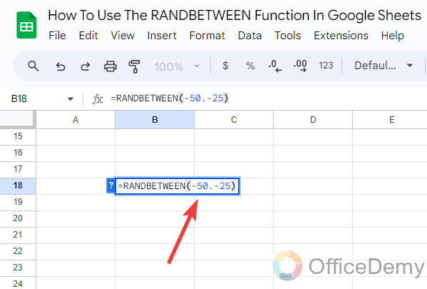
Note: Most users commit a mistake while putting an upper limit and lower limit in negative values.

Step 8

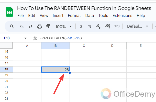
Once you have written both negative values in the RANDBETWEEN function it will give you a random negative number between the specified values as can be seen in the following result.

Step 9

Similarly, if you want to find a random number between any fraction values, you may also find it by using the RANDBETWEEN function. This time as well, you will have to be careful while putting lower limit and upper limit in the syntax as I have put in the following example.

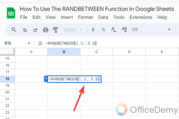
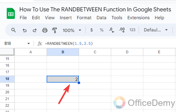
Step 10

In this way, you can get a random number between two fraction numbers in Google Sheets as well as the result below.

2. RANDBETWEEN Function with INDEX Function

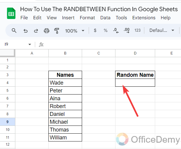
If you want to randomly select an item from any list that can be anything, any name, any fruit, any product, any grocery, etc. You can select it randomly with the help of the combination of the RANDBETWEEN function, INDEX, and CountA function in the formula that is defined as follows.

Step 1

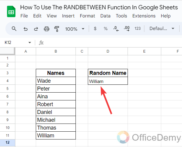
In the following sample data, we have a list of different names in the column where I have to select a random name in the following highlighted cell.

Step 2

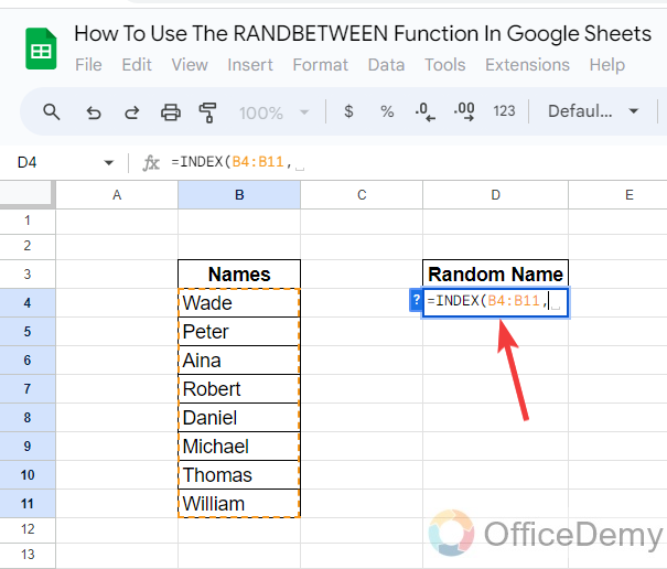
Place your cursor in the cell and run the “INDEX” function first on Google Sheets as I have written in the following picture.

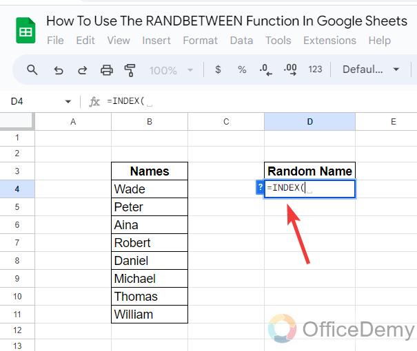
Step 3

For the INDEX function, here we will provide the address of the data range that is “B4:B11” in the following example for names as can be seen below.

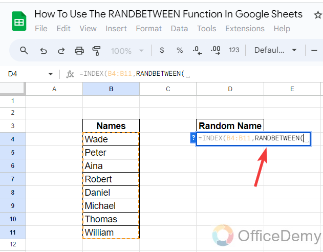
Step 4

After giving the data range of names, we will start the “RANDBETWEEN” function of Google Sheets by simply writing “RANDBETWEEN” into the syntax.

Step 5

According to the formula of the RANDBETWEEN function, here for the lower limit, we will use “1” and for the upper limit, we will use the “COUNTA” function with the data range of names as written in the following picture.

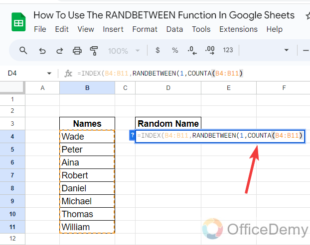
Final Formula: =INDEX(B4:B11,RANDBETWEEN(1,COUNTA(B4:B11)))

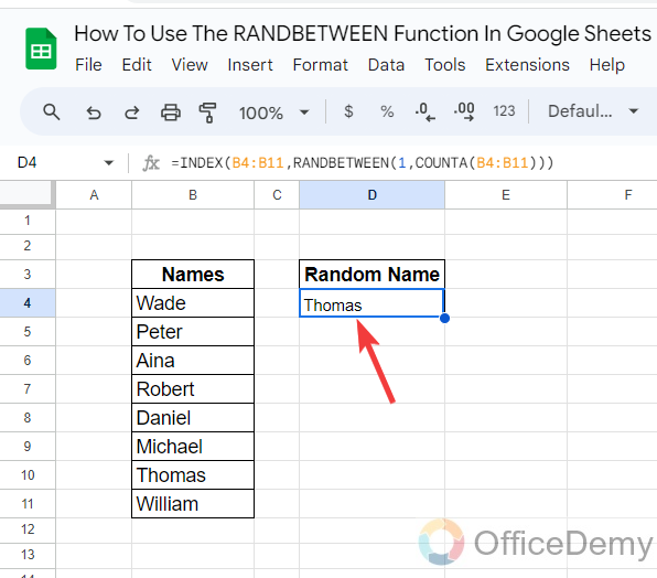
Step 6

Your syntax has been completed to select a random name from the list, now just press the Enter key and get the result as highlighted in the following picture.

3. RANDBETWEEN function with CHOOSE Function

By using the RANDBETWEEN function with the CHOOSE function, you can find a random item with an array or dataset in the syntax, or you can also write the cell reference of the values in the syntax to choose randomly. Let me show you practically with the help of the following examples to use the RANDBETWEEN function with the CHOOSE function in Google Sheets.

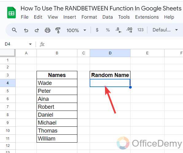
Step 1

First place your cursor where you want to choose the random names from the list with the help of using the combination of RANDBETWEEN and the CHOOSE function of Google Sheets.

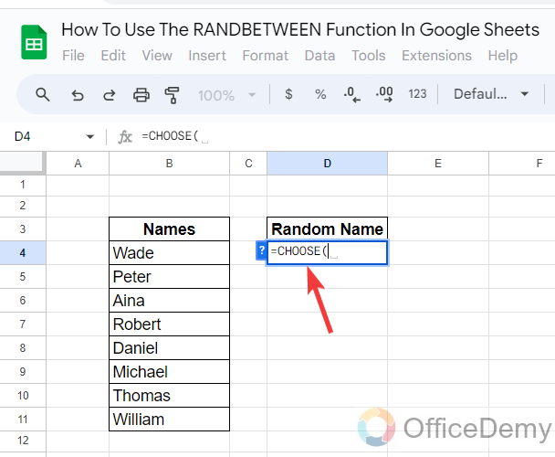
Step 2

Firstly, write the “CHOOSE” to start the CHOOSE function in the cell with an equal sign as I have written below.

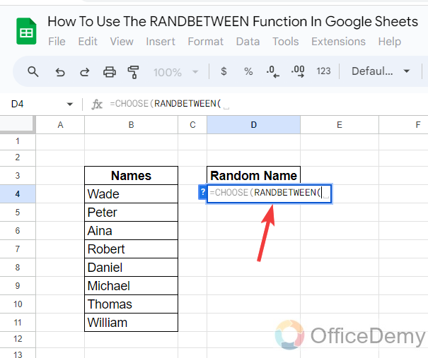
Step 3

Just after starting the “CHOOSE” function, run the “RANDBETWEEN” function as well after a small bracket has been written in the following pattern.

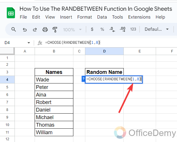
Step 4

After starting the RANDBETWEEN function, specify the upper limit and lower limit according to the number of names, as there are ten names in the list so here we have written 1,10.

Step 5

After giving the lower limit and upper limit, close the bracket and give the cell reference of each name individually separated by a comma sign as written in the following picture.

=CHOOSE(RANDBETWEEN(1,8),B4,B5,B6,B7,B8,B9,B10,B11,)

Step 6

Here, you are done now, just press the Enter key and get the random name from the list as I have gotten in the following example.

Frequently Asked Questions

Why do we get the #NUM error while using the RANDBETWEEN function in Google Sheets?

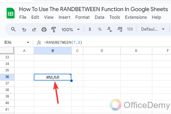
Most users complain that we usually get the #NUM error while using the RANDBETWEEN function in Google Sheets, it is because we give the lower limit an upper limit in the RANDBETWEEN function. According to the syntax, there is always a lower limit first and then shall write the upper limit. If you do it wrong, then you may get the #NUM error while using the RANDBETWEEN function in Google Sheets as you can see in the following demo.

Step 1

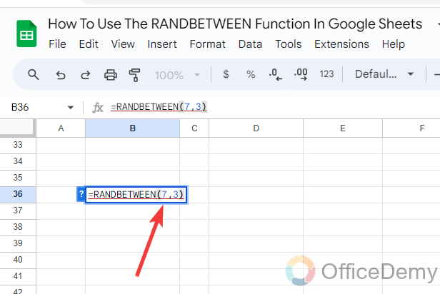
According to the formula of the RANDBETWEEN function, we write first the lower limit in the syntax and then the upper limit but if you write it wrong that first upper limit and then lower limit as I have written in the following example.

Step 2

In such a situation we get a “#NUM” error while using the RANDBETWEEN function in Google Sheets.

Conclusion

Hopefully, you have understood the usage of the RANDBETWEEN function with the above guide on how to use the RANDBETWEEN function in Google Sheets. Now you can find a random number according to your desire instead of a value between 0 and 1.