How to Create a Grid Chart in Google Sheets

Hi, today we will learn how to create a Grid Chart in Google Sheets. Earlier for several years, no one knew about the grid chart but now it is being used to represent data in reports. The grid chart is a visualization option for displaying data, which presents the information in a matrix. Unfortunately, there is no direct way to create a grid chart in Google Sheets, most users get stuck into trouble while creating a grid chart in Google Sheets therefore I have brought a topic on how to create a grid chart in Google Sheets in which we will learn a hack for creating a grid chart in Google Sheets.

Advantages of a Grid Chart in Google Sheets

Visualization of grid charts helps the user to display data and present the information in a matrix form. The analysis of a grid chart is very helpful in unnecessary data items from reports. It can also be used for identifying the responsibilities of various managers for a particular system. You can define a relationship between two different sets of factors in a tabular method. If you are having trouble creating a grid chart in Google Sheets, then follow the following instructions to create a grid chart in Google Sheets.

Step-by-step Procedure – How to Create a Grid Chart in Google Sheets

Unfortunately, there is no direct way to create a grid chart in Google Sheets, but Office Demy has always been the solution to accomplish any task. So here as well, we have found a way to create a grid chart in Google Sheets. Follow the following steps to create a grid chart in Google Sheets.

Step 1

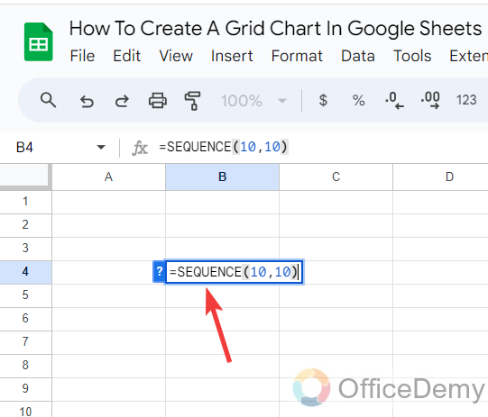
To make a grid chart, I am taking a sequence of 10 by 10 in Google Sheets. To make a sequence of 10 by 10, here I am using the SEQUENCE function of Google Sheets and entering the “10,10” in the arguments for the 10 by 10 order.

Step 2

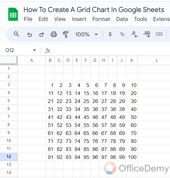
As I press the Enter key, we will get the result as follows. As can be seen below here we have gotten the sequence of 1 to 100.

Step 3

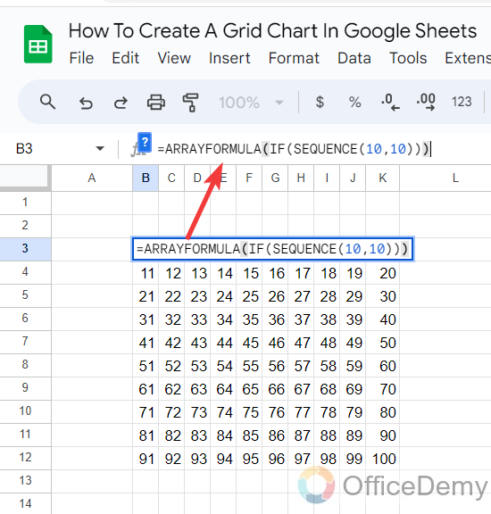
In cell A1, we will add a value later through which values will be changed accordingly. For that, I am adding the IF function along ARRAY FORMULA function into the syntax as can be seen below

.

Step 4

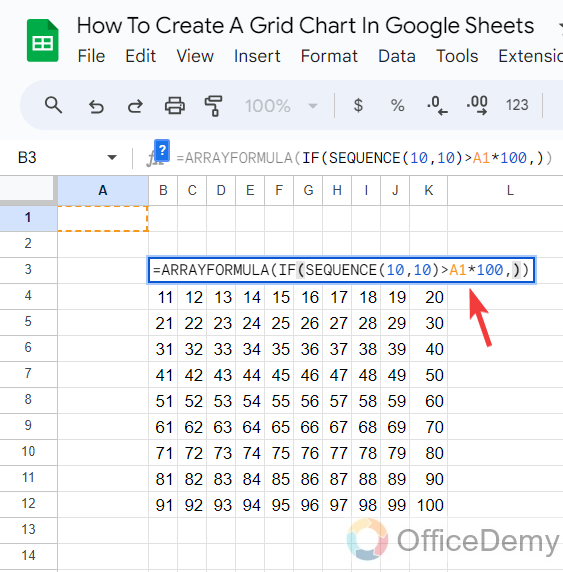
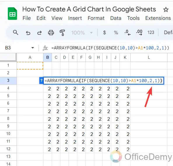
For the IF function, I am using a condition as written in the following syntax “Sequence(10,10)>A1*100“, that means if the value in sequence is greater than the value in the cell A1 then multiply it by 100.

Step 5

Now, we will specify the value of true or false where I am writing “2” for true and “1” for false as you can see the syntax in the following example.

Step 6

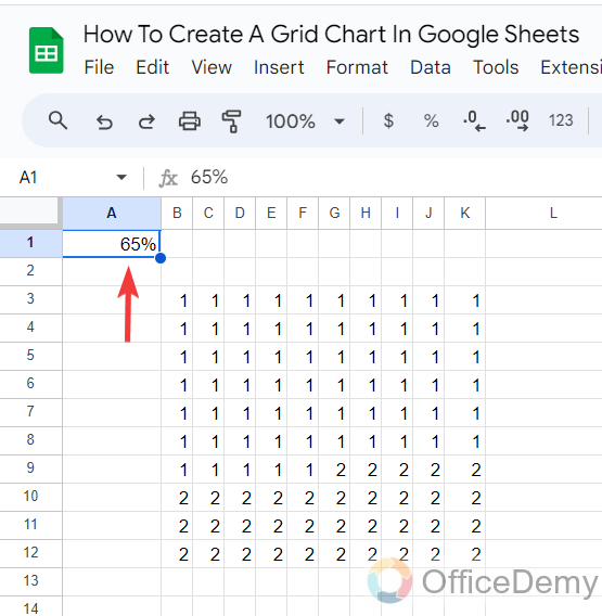
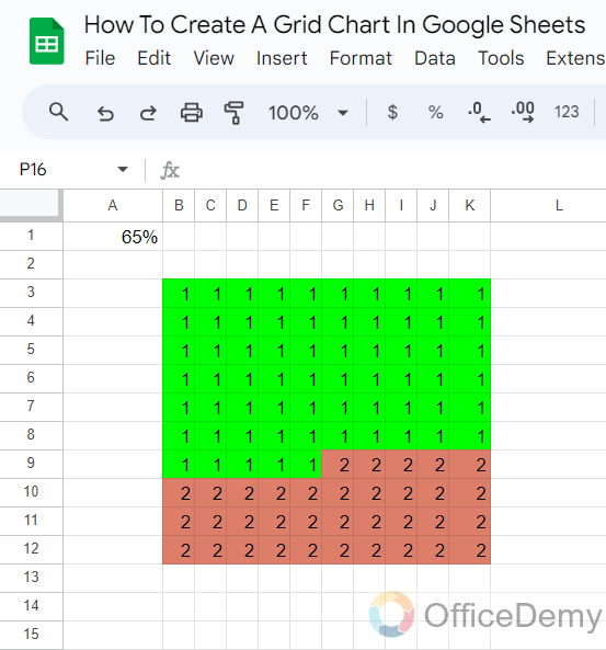
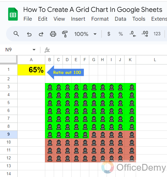
Now, let’s put the value in cell A1, for example, here we are putting the value “65%” in the following example. In this way, we will get 65% different values and the rest of the 35% will be different as given as you can see the result in the following picture.

Step 7

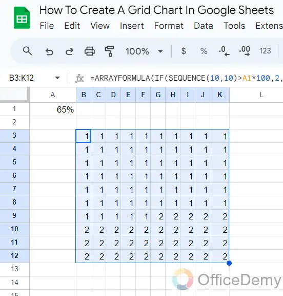
To make a grid chart on these numbers, let’s apply some conditional formatting. To apply Conditional formatting, first select all the ranges as I have selected below.

Step 8

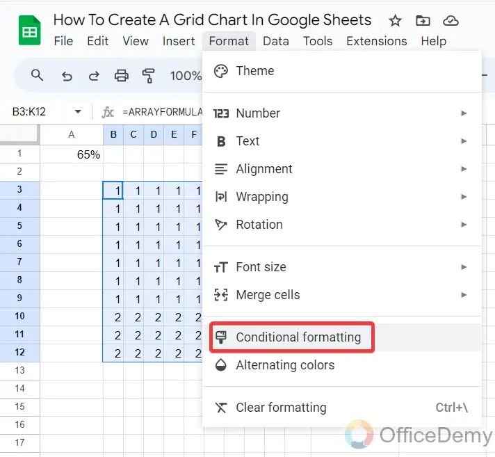
After selecting the range, go into the “Format” tab from the menu bar of Google Sheets, a drop-down menu will open where you will see the “Conditional formatting” option as highlighted below.

Step 9

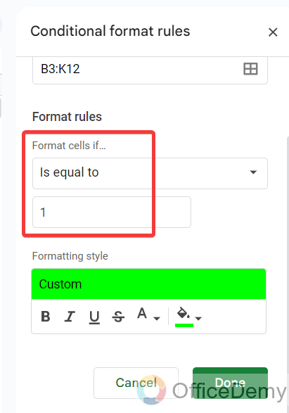
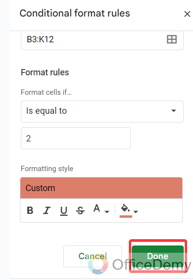
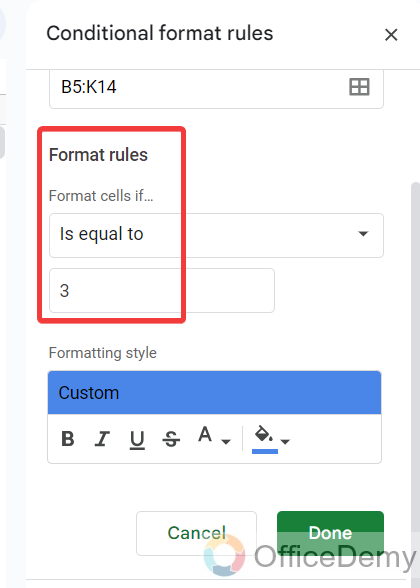
Clicking on the “Conditional formatting” option will give you a pan menu at the right side of the window, set the format rule to “Is equal to” and write the value “1” in the dialogue box as highlighted in the following picture.

Step 10

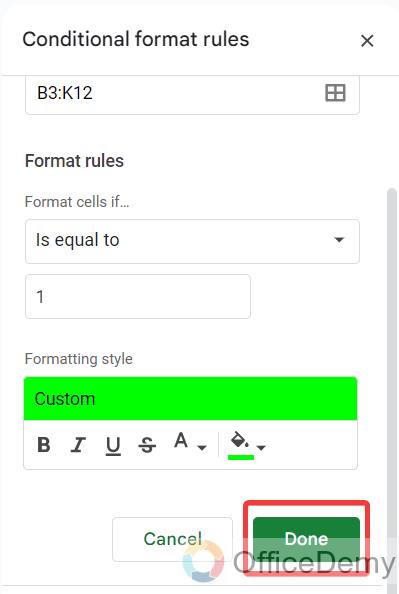
For these format rules, I have selected the color fill with “Green” as can be seen below, after setting formatting simply click on the “Done” button to apply this conditional formatting.

Step 11

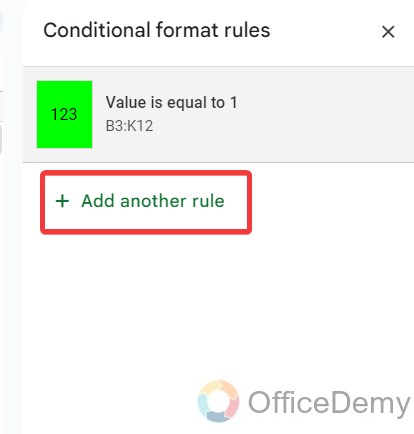
As we have two values in our data range here, we will add another conditional formatting for the second value. To add another conditional formatting, click on “Add another rule” from the pane menu as highlighted below.

Step 12

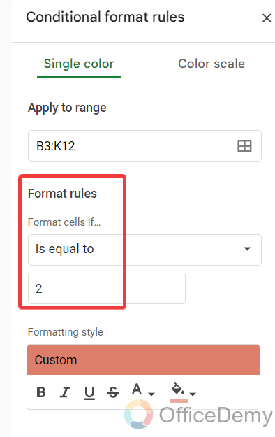
Again, set the format rule to “Is equal to“, previously we had written “1” so this time I have written “2” in the dialogue box to apply the conditional formatting on the cell containing “2“.

Step 13

For the cells that contain “2“, I have chosen the color “Red” to make a grid chart in Google Sheets, now just simply click on the “Done” button to apply this formatting.

Step 14

Once you have applied both conditional formatting, you should get the results like this as can be seen in the following picture.

Step 15

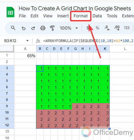
As we are creating a grid chart in Google Sheets, here we will format the numbers as a bust in silhouette emoji. To format cells, go into the Format tab of Google Sheets but don’t forget to select all the cells before going into the Format tab.

Step 16

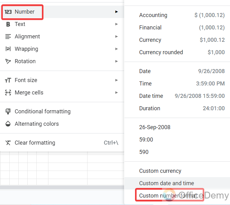
When you click on the “Format” tab from the menu bar a drop-down menu will drop down, click on “Number” then click on “Customs Number Format” as highlighted in the following picture.

Step 17

As you click on “Customs Number Format“, a small pop-up window will open in front of you, copy a bust in silhouette emoji from a web paste in the number format dialogue box and then click on the “Apply” button.

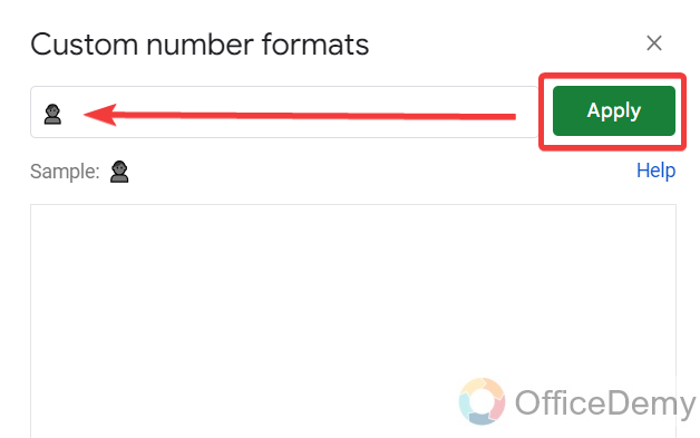
Step 18

Now, when you go back to the chart, you will see all your numbers bust in silhouette emoji as required. The Grid chart is ready now, in this simple way you can create a grid chart in Google Sheets.

How to Create a Grid Chart in Google Sheets – FAQs

Q: How to make a three-color grid chart in Google Sheets?

A: In the above tutorial we have created a grid chart in Google Sheets with two values but if you want to create a grid chart with three different colors or three different values, you can also create it by just adding one more condition in the syntax. In this way, you will get three different values in the data range that you can format with different colors to make a three-color grid chart in Google Sheets. Let me show you practically in the following steps.

Step 1

First, we will apply a three-condition formula to generate three types of numbers in the sequence with the help of the following formula.

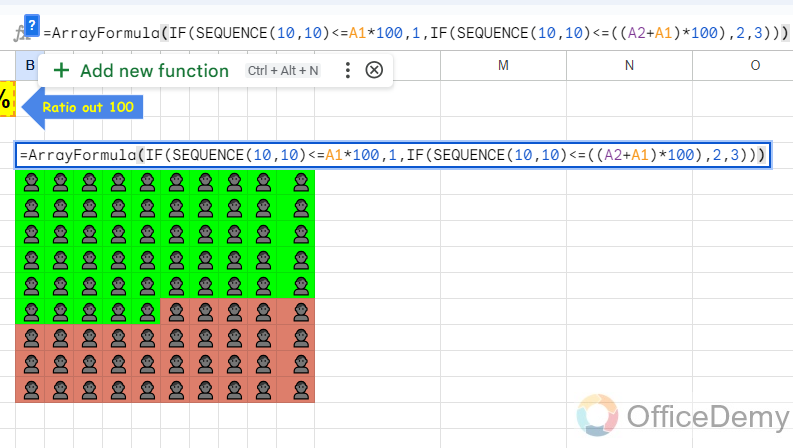
Formula:

=ArrayFormula(IF(SEQUENCE(10,10)<=A2*100,1,IF(SEQUENCE(10,10)<=((A3+A2)*100),2,3)))

Step 2

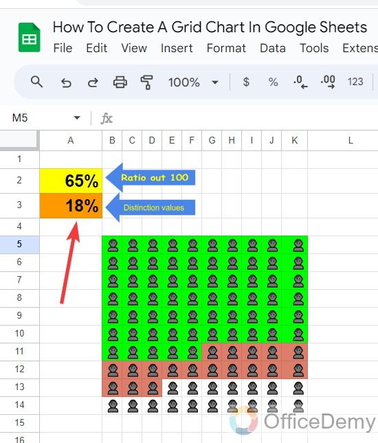
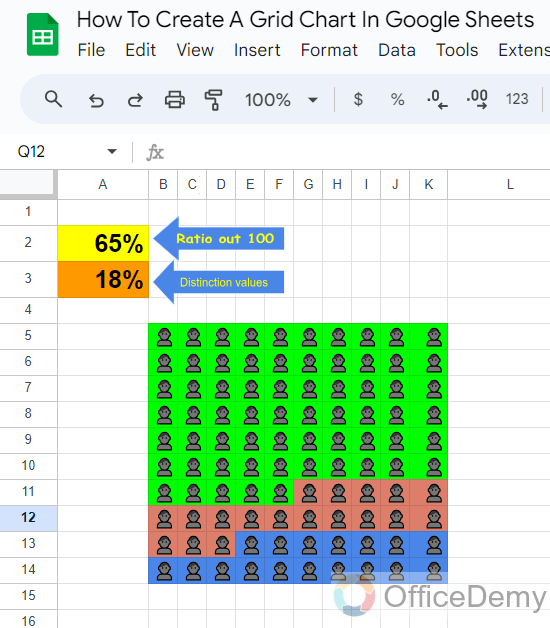
The third value will be generated by putting the value in cell A3, as much as you want to generate the section of third values. As I have written “18%” in the following example. In this way you will get 65% values of 1, 18% value of 2 and the rest of the values will become 3.

Step 3

Now, we will again apply the conditional formatting for the value of “3” as We have applied above. Here I am using blue for the third value.

Step 4

As you click on the “Done” button, the three colors of the grid chart are ready in front of you as you can see the result in the following picture.

Conclusion

Hopefully, you must like the above trick of creating a grid chart in Google Sheets as there was no way to create a grid chart in Google Sheets. We hope that soon we will get an option for creating a grid chart in Google Sheets by Google Workspace. Till then you can get an advantage from the above tutorial on how to create a grid chart in Google Sheets.