How to Label Legend in Google Sheets [Guide 2023]

Google Sheets is a spreadsheet software therefore graphs and charts in Google Sheets can be extremely valuable for visualizing data, but just displaying a chart with a bunch of columns or lines of different colors is not enough. In this case label legends are very useful to introduce the users to clear their confusion. If you want to label legends to your chart, then fortunately Google Sheets makes it easy to do this.

This tutorial will show you how to label legends in Google Sheets. Let’s start our topic without wasting our time.

Importance of using Label Legend in Google Sheets

When you are dealing with the visualization of data in Google Sheets through any chart or graph then it is necessary to make sure that the person looking at your chart should be aware to gain insight into what they are displaying.

That’s why it is compulsory to include a label legend with your chart that tells the user what each of these lines, shapes, or colors are describing. We can say a chart without labels, a clock without its needles. I recommend you not forget to add label legends to your chart. Read the following article and learn how to label legends in Google Sheets.

How to Label Legend in Google Sheets

The method of labeling legends in Google Sheets is quite easy. You can label legends with just a few clicks if you have a chart. In this tutorial, I will give you two examples of the different charts in which we will learn how to label legends in Google Sheets.

How to Label Legend in Google Sheets – In Pie Chart

Step 1

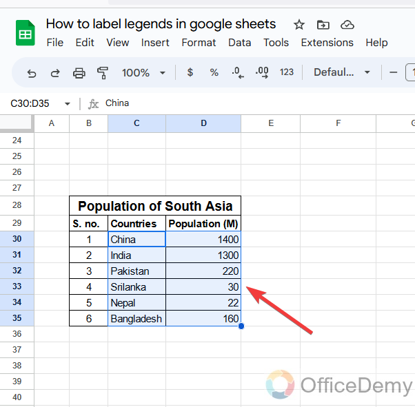
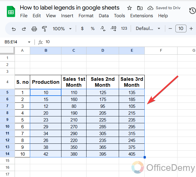
Let’s suppose this is your sample data, first, select the values to insert a chart.

Step 2

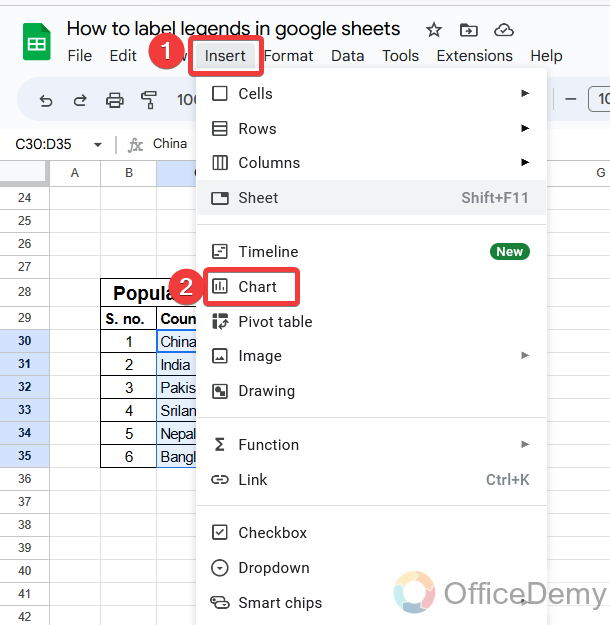
To insert a chart, go into the “Insert” tab of the menu bar of Google Docs, and a drop-down menu will appear where you can find a “Chart” option. Click on it to insert it.

Step 3

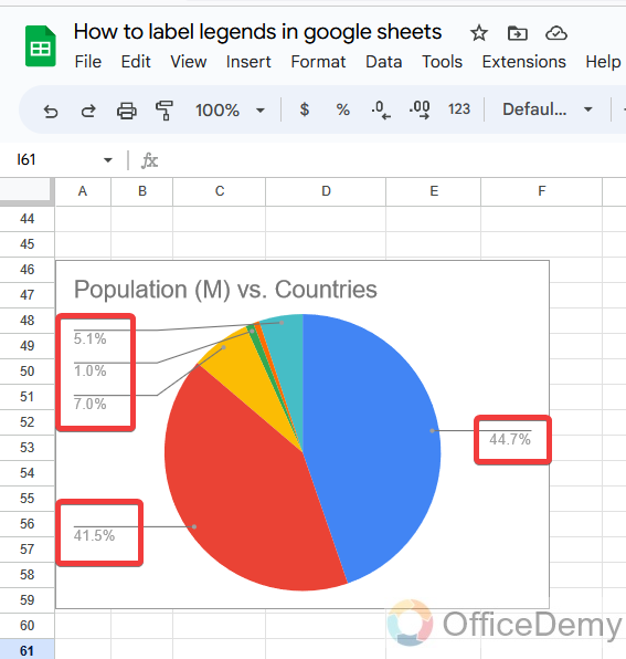
As you can see in the following picture that our chart has been inserted, and you can also see the legends highlighted along the chart. But unfortunately, we don’t have labels with the legends. Let’s insert it.

Step 4

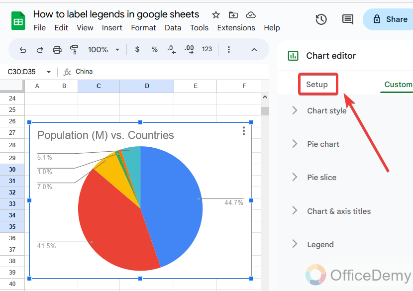
When you click on a chart, a chart editor will open at the right side of the window, where you go into the chart “Setup”

Step 5

When you open the chart setup, several options will appear in which you can see the “Label” option through which you can label legends in Google Sheets.

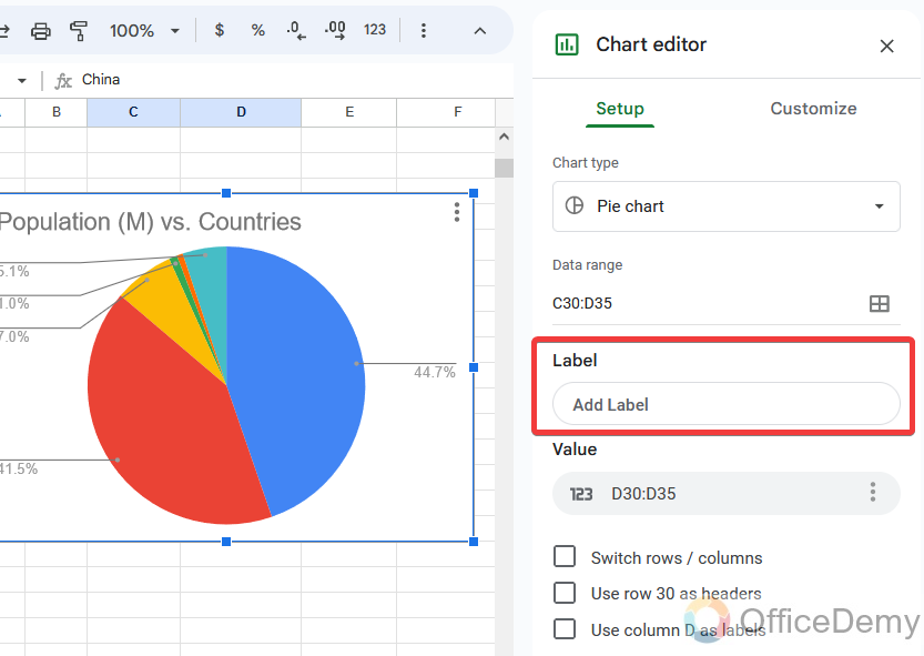
Step 6

When you click on “Add label“, it will ask you to select the data range. Click on the following option to give the data range.

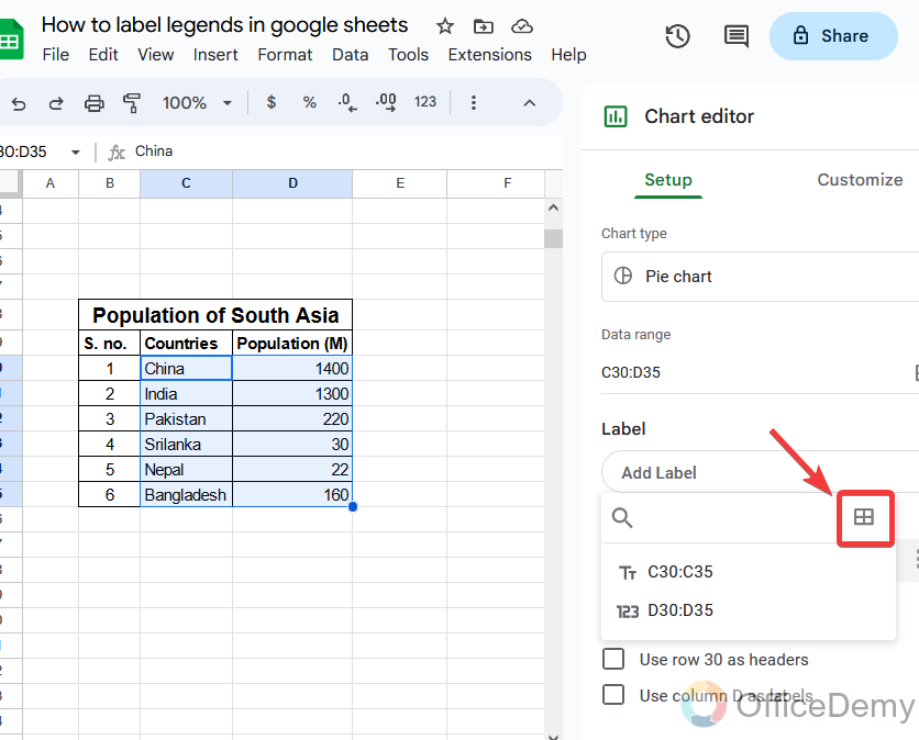
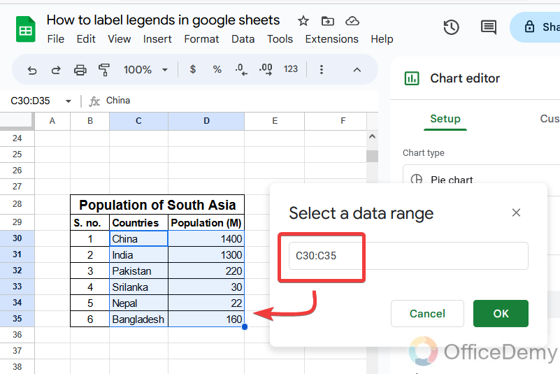
Step 7

When you click on the data range option, a new pop-up window will open where you will have to give the data range and then press the OK button.

Step 8

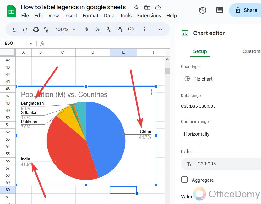
As you click the OK button, you will see your legends labeled in the chart. As you can see in the following picture.

In this way, you can add label legends in Google Sheets.

How to Label Legend in Google Sheets – In Bar Graph

Step 1

Let’s suppose this is our sample data for creating a bar graph. To insert a chart first select your data then go into the “Insert” tab of the menu bar, then click on the “Chart” button from the drop-down menu.

Step 2

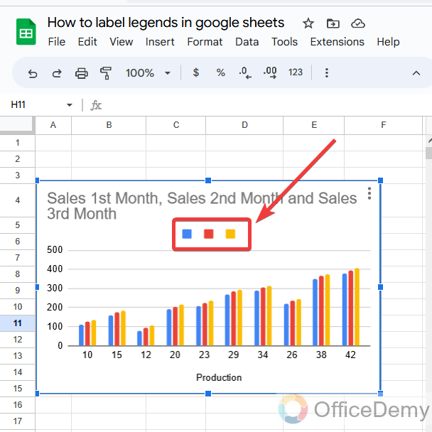
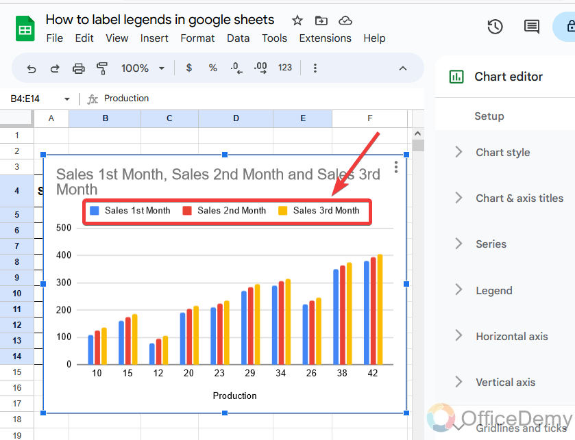
Here we have got our chart as you can see in the following picture. It also has legends attached to the top of the chart as highlighted in the following picture. But in the following chart we also don’t have labels with the legends so let’s insert them.

Step 3

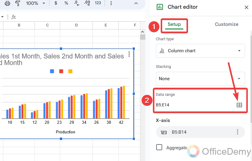
First, access the chart editor from the three dots of the chart, then go into the chart Setup from the side pan menu of the chart editor. In the chart, setup finds the “Data range” option to give the range of your chart.

Step 4

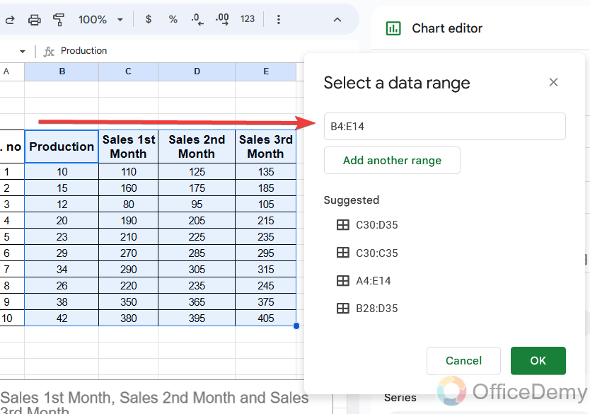
When you click on date range, it will ask you to select the range, then select the range of your chart values including headers because we will use these headers as a label in the chart as I have selected the range you can see the following example.

Step 5

When you get done with giving the data range, simply click on the OK button present in the same pane menu. As you will click on this OK button, you will instantly see your labels with the legends as shown below.

Frequently Asked Questions

Q: How to change the position of labeled legends in Google Sheets?

A: We have learned how to label legends in Google Sheets. But by default, Google Sheets usually place this label at the top of the chart. However, we may need to change its position. Let’s suppose you have legends at the top of the chart, and you want to place it on the right side of the chart then don’t worry Google Sheets provides features according to their user’s desires. These are the following steps through which you can change the position of labeled legends in Google Sheets.

Step 1

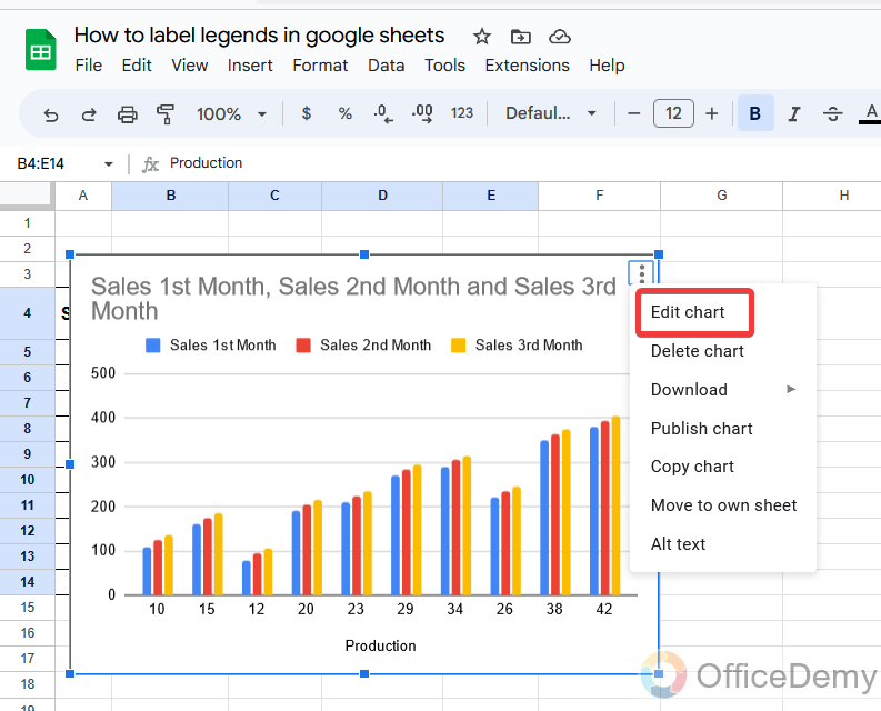
The first thing you need to do is open the chart editor, which you can open from the three dots option at the right top of the chart. When you click on it a small menu will drop down where you will see the “Edit chart” option at first. You can open the chart editor by clicking on it.

Step 2

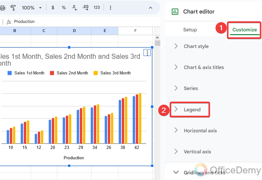
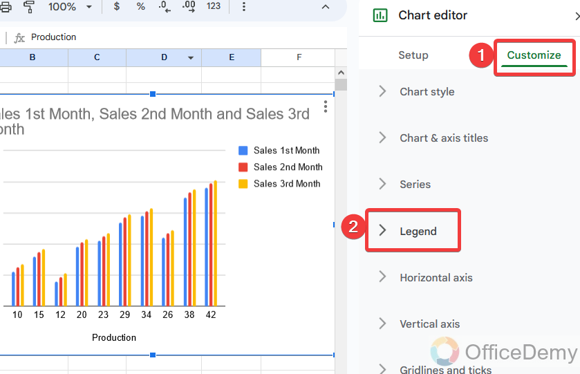
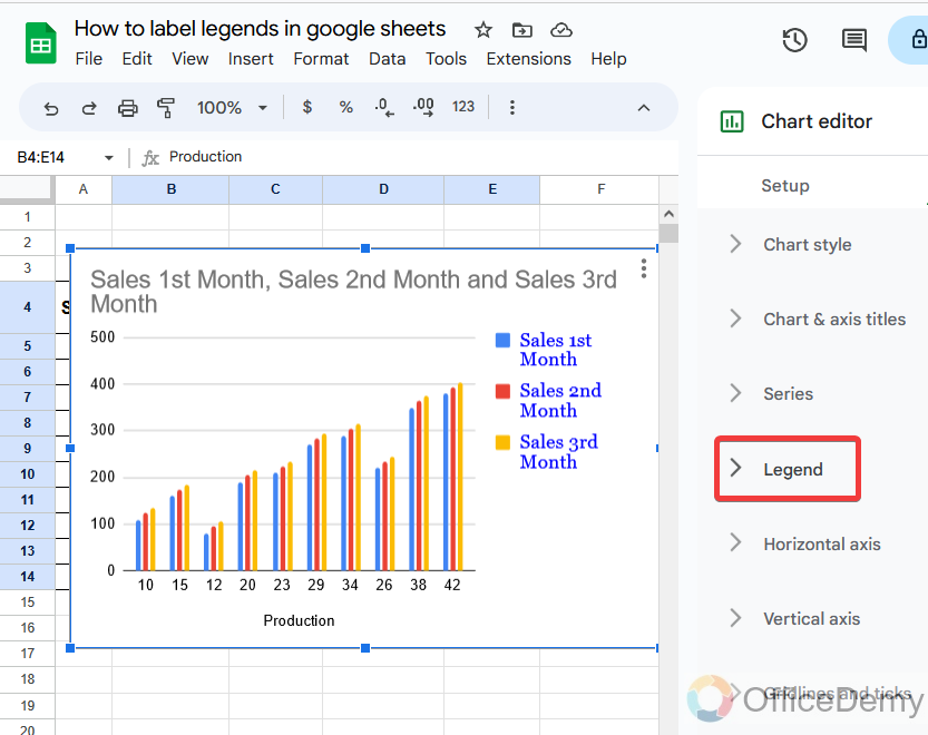
As you click on the Edit chart, a side pane menu will appear at the right side of the window where you will have to go to “Customize” and then “Legend” from the listed menu as shown below.

Step 3

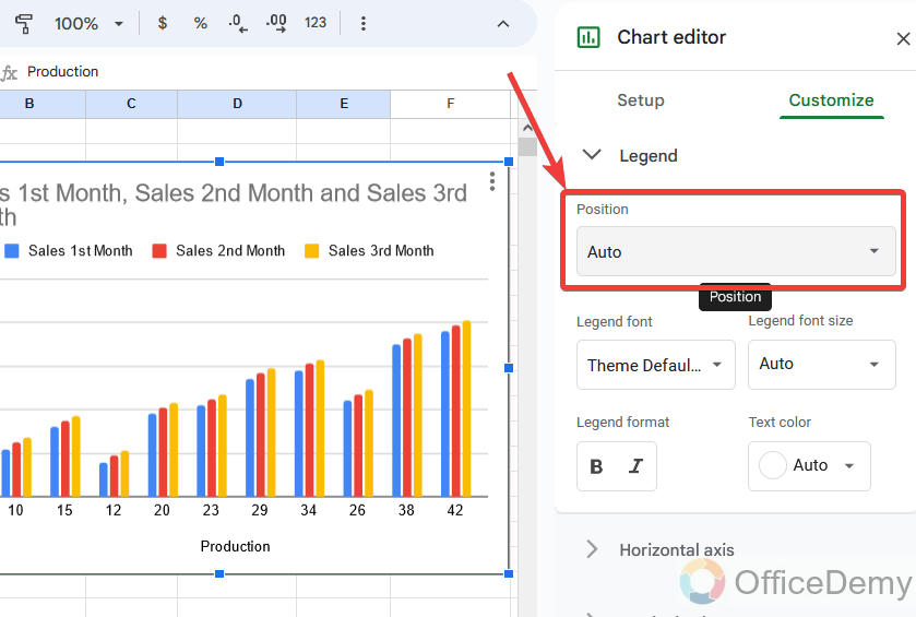
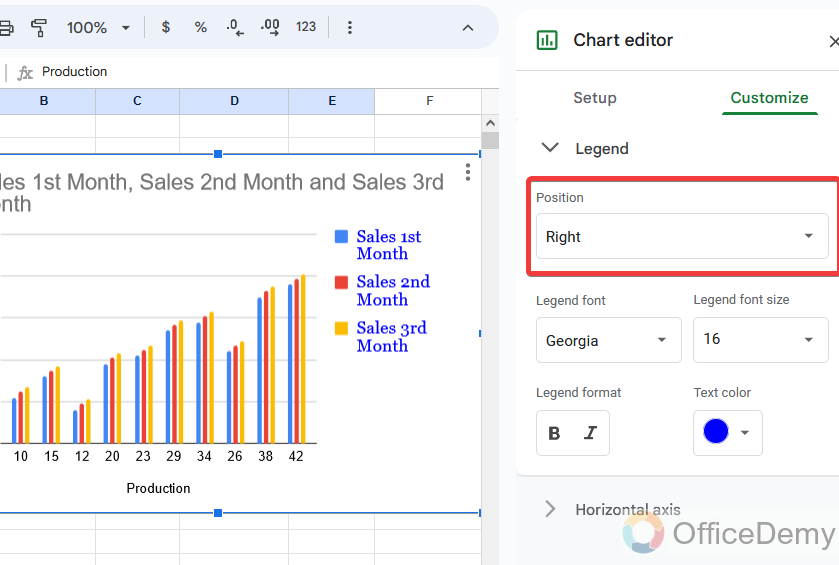
Clicking on this Legend button will give several formatting options, but at first, you will find the option for positioning the legends. With the help of this option, you can move your legends anywhere along the chart. Let’s open it to see.

Step 4

Yeah! You can see the options in the following picture, there are directions given to move your legends. As we need to move our legends toward the right side of the chart let’s select the “Right” option.

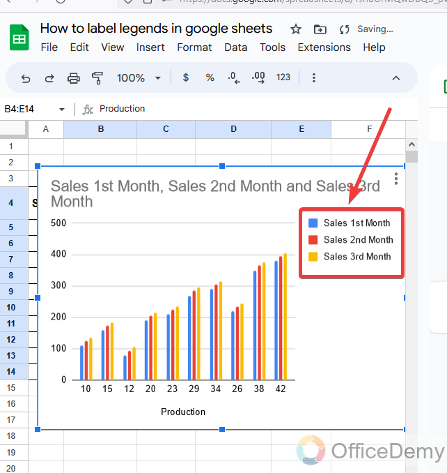
Step 5

Here we got the results as can be seen in the following picture, legends have been moved towards the right side of the chart as required with their labels as well.

In the same way, you can move these legends anywhere along the chart according to the given criteria.

Q: How to format the label legends in Google Sheets?

A: If you were surprised to know that you can label legends in Google Sheets then this is more exciting for you that you cannot only label legends in Google Sheets but also can format them according to your wish. If you want to make an attractive chart and labels are spoiling the stylish look of your chart or graph. Then make your labels stylish too. Yes, with the help of the following steps you can format your label legends in Google Sheets.

Step 1

To format label legends as well we will have to go into Customize and then Legend as above.

Step 2

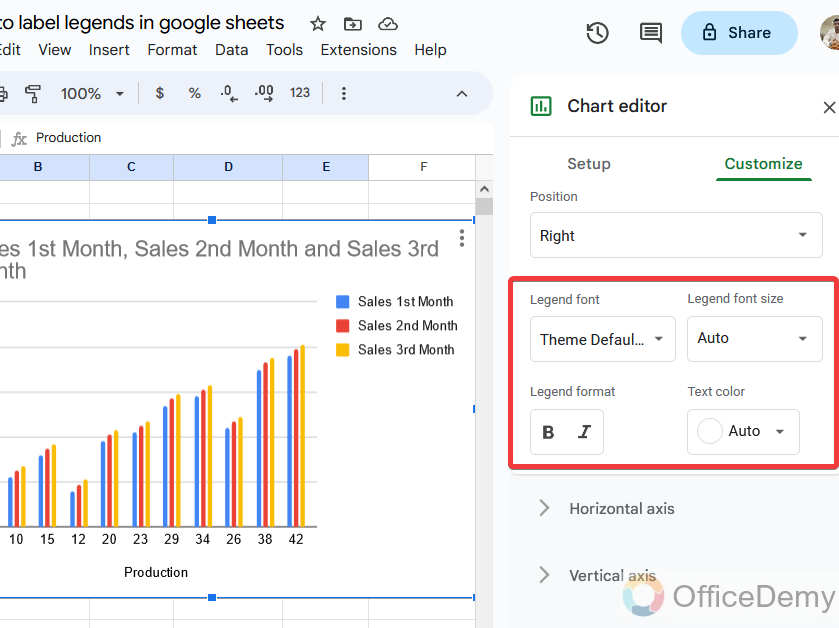
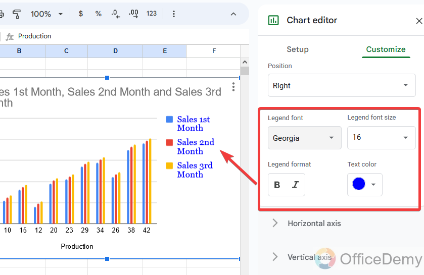
Where you will get some formatting options through which you can edit font size, font style, and font color and can also perform the operations of Bold and italic to your label from these options.

Step 3

As you can see the result in the following picture in which I have changed the font style, size, and color as well with the help of these options. Similarly, you can also format your label legends in the following way and can get the desired results.

Q: How to remove the label legends in Google Sheets?

A: I hope you have gotten to label legends in Google Sheets, but maybe somewhere you may need to remove them, then what will you do? So do not get to worry if you ever need to remove these label legends then here is the way you can remove label legends in Google Sheets.

Step 1

Go into the “Legends” from the chart editor menu in the Customize section.

Step 2

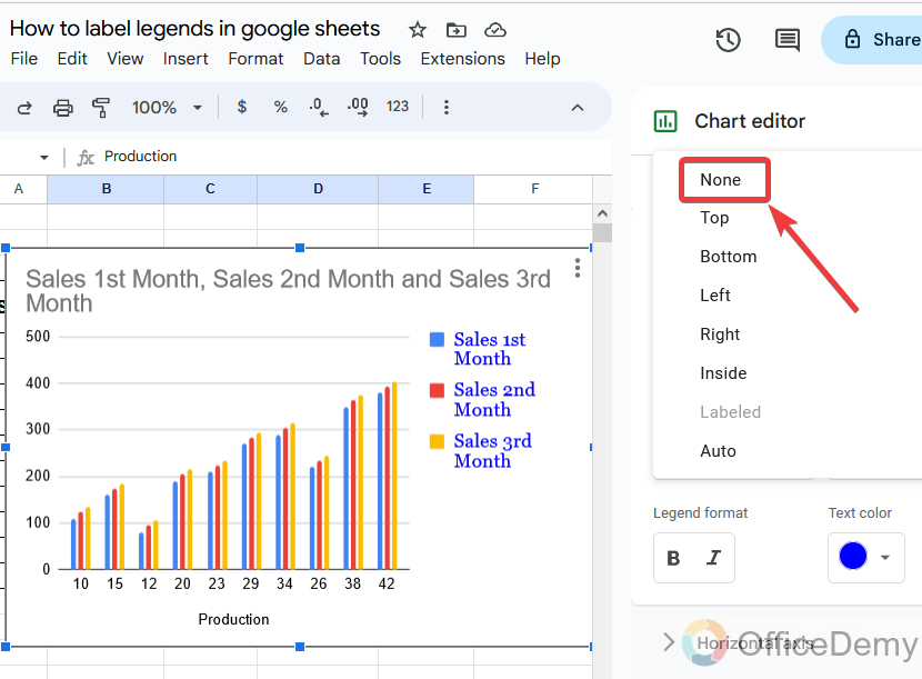
Then follow the option from where we changed the position of labeled legends as shown below.

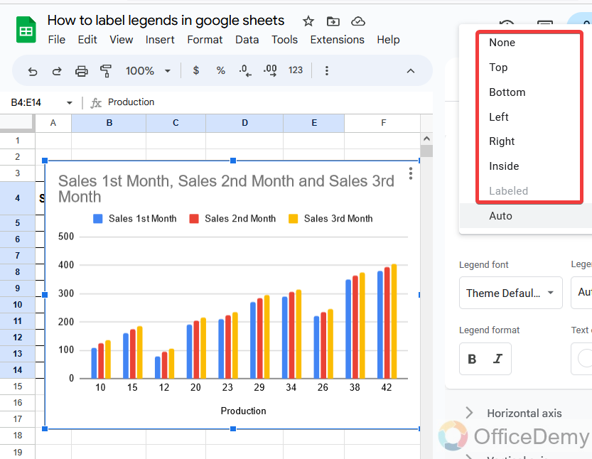
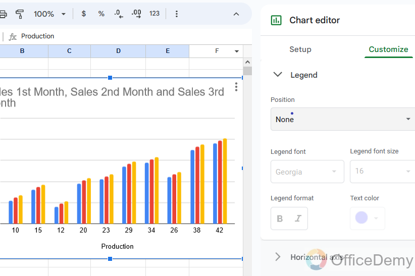
Step 3

When you open this option, you will find a “None” option at the first. You can remove your label legends by selecting this option. Just click on it.

Step 4

As you can see the result in the following picture, our label legends have been removed from the chart.

Conclusion

Today we learn how to label legend in Google Sheets. Readers attract the material that is easy to understand but a chart or graph without label legends is much more difficult to understand. Therefore, the above article on how to label legends in Google Sheets can give you a way to provide your readers flexibility. I have also covered how to format legends, the position of legends, and how to remove them which will also be very useful.