How to Make an Attendance Sheet in Google Sheets [Full Tutorial]

Let’s learn how to make an attendance sheet in Google Sheets. If we look several years behind, attendance sheet making was limited to just a piece of paper and that too manually used to be costly and time-consuming especially while calculating the total attendance for the students or attendance percentage.

But now with the help of Google Sheets, you can create an amazing attendance sheet template within a few minutes with automatic rules and functions. Leave the words and go through the following tutorial on how to make an attendance sheet in Google Sheets.

Benefits of Making an Attendance Sheet in Google Sheets

The biggest benefit of making an attendance sheet in Google Sheets is its functions that can automate your attendance sheet and can make any calculation within seconds.

Secondly, Google Sheets has enough drawing tools and conditional formatting features through which you can give a creative & colorful layout to your attendance sheet. Making an attendance sheet in Google Sheets is such a save of time and free of cost.

How to Make an Attendance Sheet in Google Sheets

There is no technical procedure for making attendance sheets in Google Sheets, it’s totally up to you what you want to add to your attendance sheet. Google Sheets has effective tools to create an attendance sheet template and enough functions to track an attendance sheet. Let me show you a making template with the help of Google Sheets tools and rules.

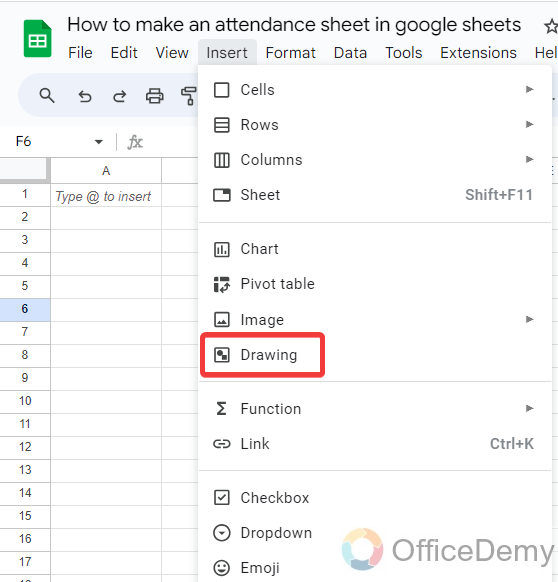
Step 1

Here I am going to insert the Attendance Sheet title first for which I am taking the drawing tool of Google Sheets from the Insert tab as highlighted in the following screenshot.

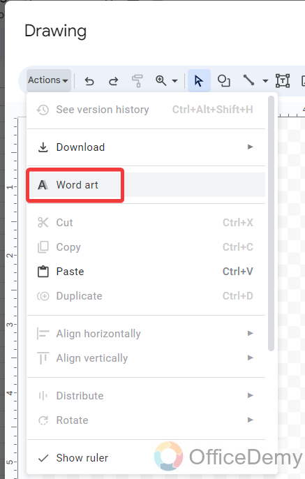
Step 2

When you click on the “Drawing” tool, a separate window will open in front of you. On this window, click on the “Actions” button where you will see “Wordart“.

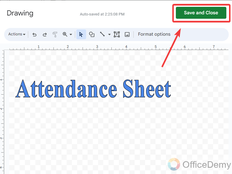
Step 3

Prepare your Attendance Sheet title by formatting styles, font, text fill color, etc. Once you have completed creating your Attendance Sheet title click on the “Save and Close” button.

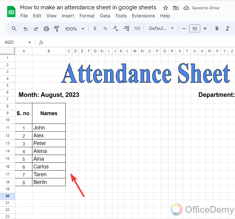
Step 4

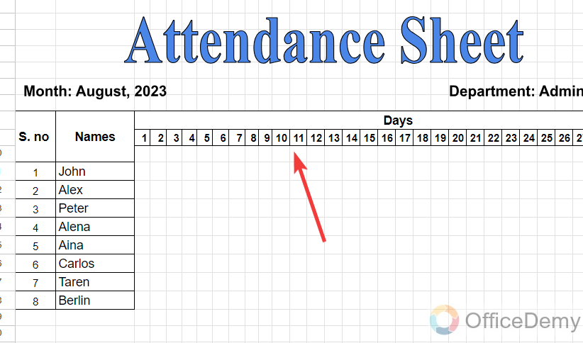
After inserting the title name, you may also add subheadings for the month, department, etc. In the attendance sheet in the first column, we will add the names of candidates or participants for whom you are making the attendance sheet.

Step 5

After adding the names to your attendance sheet, in the second part, we will add the dates for a whole month, as we are making a monthly attendance sheet here, we have inserted dates from 1 – 31 as can be seen in the following picture.

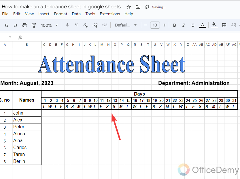
Step 6

Along with the dates, we will insert the day’s column as well so we will find the holidays as well. Adjust all columns to make them fit so they won’t occupy more space. As I have made in small blocks in the following example.

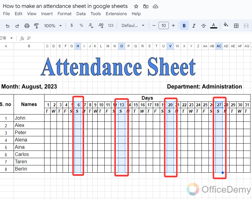
Step 7

As we all know, Sunday is a holiday in most of the regions so obviously those cells would remain empty so, Let’s differentiate them by filling color. To fill with color, first select all the days regarding Sunday.

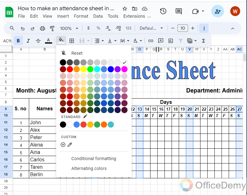
Step 8

After selecting the box that we need to fill with color, click on the “Fill color” icon, and a drop box will drag down to the color gallery. Select the color with which you want to fill the boxes.

Step 9

The result is in front of you, as you can see in the following picture, Now we can know the days containing Sundays are highlighted in the attendance sheet.

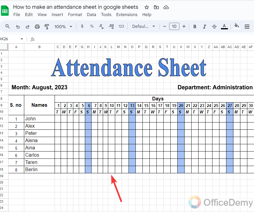
Step 10

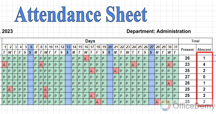
The structural attendance sheet is ready for now, you can take attendance day-by-day putting simply “P” for present and “A” for absent.

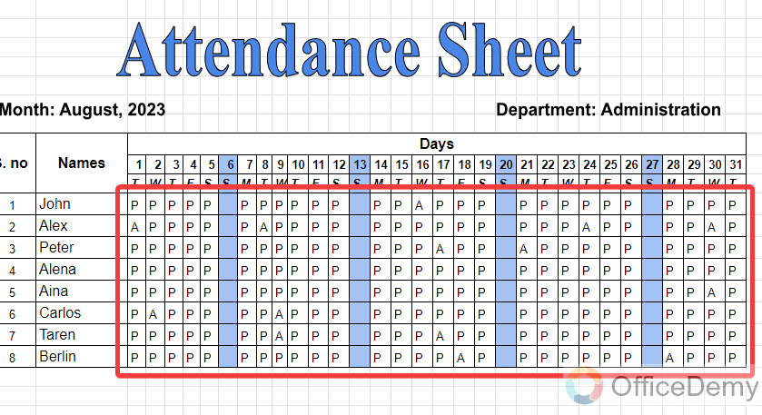
Step 11

If you look at this attendance sheet, it is very difficult to find out when someone is absent. Don’t worry, I will tell you an effective way to find out. First, select all the cells containing attendance as I have selected below.

Step 12

After selecting the range, go into the “Format” tab from the menu bar then click on the “Conditional formatting” option when a drop-down menu opens.

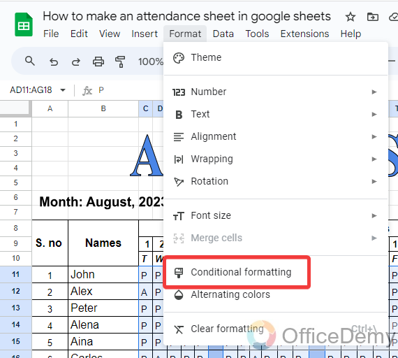
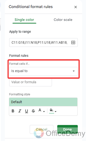
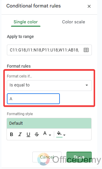
Step 13

When you click on “Conditional formatting“, a pane menu will appear on the right side of the window. Firstly, apply the “Format rule” to “Is equal to” from the following highlighted picture.

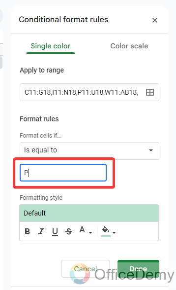
Step 14

Now, we will put the value “P” in the following highlighted which means it will create a rule that formats the cell when the cell is equal to “P“.

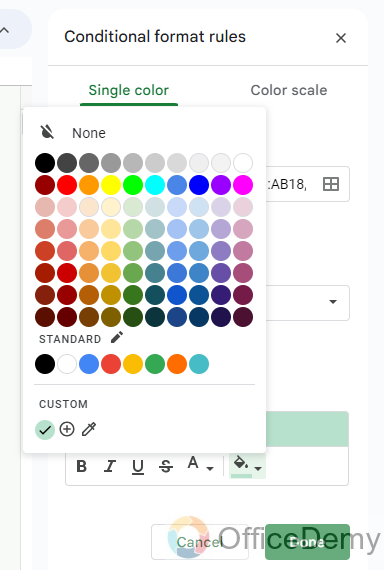
Step 15

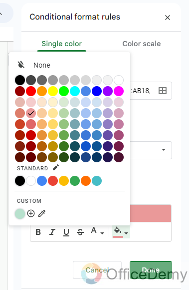
Here, I am applying the formatting just to fill the cell with a “Green” color. You may also choose according to your preference.

Step 16

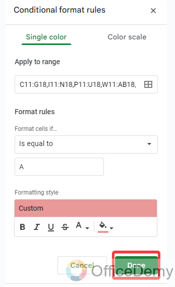
Once you have completed formatting the cell, then click on the “Done” button to save the rule.

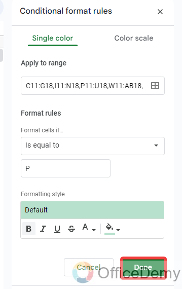
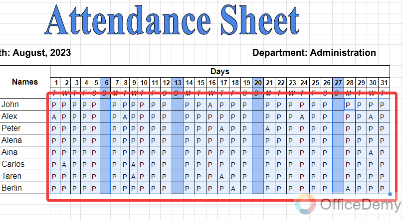
The above rule will format your cell with a green color when it is equal to “P” or present.

Step 17

In the same way, we will create a rule for the absent people. Similarly, again select the “Format rule” to “Is equal to” and now we will write “A” to recognize the absent cells.

Step 18

In this rule, I will mark absent cells with the red color so here I will select the “Red” color to highlight the cell containing absent.

Step 19

Again, simply click on the “Done” button after completing the rule as highlighted in the following picture.

Step 20

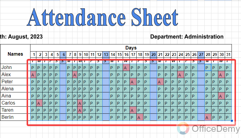
Now, see the image of the attendance after applying the formatting rule all present cells are highlighted with the green color and absent cells with the red color so we can easily indicate them.

Step 21

You are almost done with creating the attendance sheet but at the end of the month, you may need to calculate the total presence and absence of the candidates. To find total presence and absence we will use the “Countif” formula.

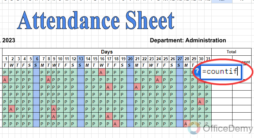
Step 22

In the COUNTIF formula first, you will have to give the cell range as I have given below.

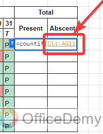
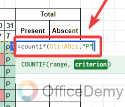
Step 23

As we are calculating total presence, here we will write “P” which means that count the cells if cells contain “P“.

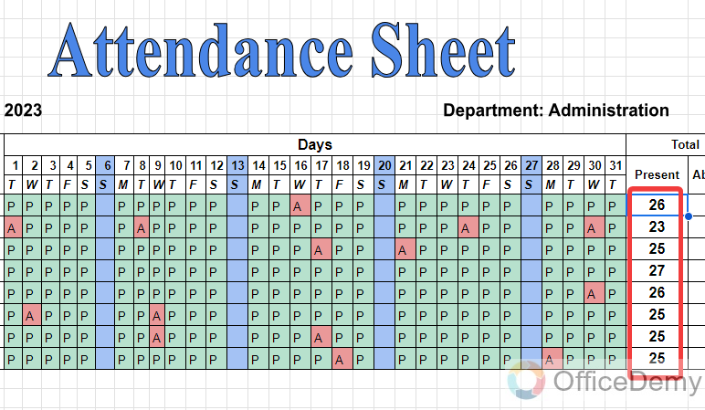
Step 24

So, we will find the total presence made by the person in a month. Simply drag the formula to find the total presence of other participants.

Step 25

Similarly, to find total absence, we will write “A” instead of “P” as written in the following picture.

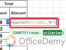
Step 26

So, we will also find the total absence for the person.

That’s all from my side, the attendance sheet has been completed, you may add or remove anything according to your preference.

Frequently Asked Questions

Can I Tag Someone in an Attendance Sheet in Google Sheets?

Q: How to find attendance percentages in Google Sheets?

A: Expressing numbers in percentages always helps you to give a better sense of proportion. As we know Google Sheets is mainly used for calculations, so finding percentages in Google Sheets is not a difficult task. Follow the following instructions to calculate the percentages for an attendance sheet.

Step 1

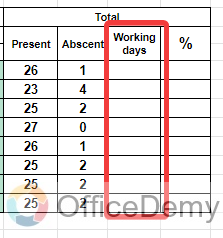
To find the attendance percentage, first, we will have to find the total working days of the month.

Step 2

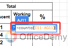
To find the total working days we will use the “CountA” formula. Counting all formulas will calculate all the cells containing a value except empty cells.

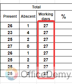
Step 3

As you can see in the result below, now we have the total number of working days in the month.

Step 4

As we know the percentage formula obt. Marks/Total number*100. In the following example obtained marks are the total presence and total numbers are the Working days of the month. Let’s apply the formula accordingly.

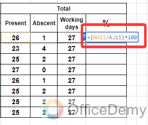
Step 5

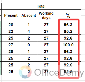
You will get the attendance percentage as can be seen in the following example.

Conclusion

Although you may find lots of pre-made attendance sheet templates if you want to make an original attendance sheet of your desire learn the above tutorial on how to make an attendance sheet in Google Sheets.