How to Use Not Equal Google Sheets Symbol

Google Sheets is a powerful tool to deal with spreadsheets with its functions and features. To make a logical expression we use operators in these functions and conditions to compare or analyze values, The Not Equal symbol is one of them in Google Sheets.

If you are not aware of this operator of Google Sheets then go through the following guide on how to use the Not Equal Google Sheets symbol.

Importance of using Not Equal Google Sheets Symbol

The main purpose of this operation is to find whether the value in a cell does not match the data value in another cell. With the help of this symbol, you can compare any kind of data or you can analyze the data whether the value exists or not.

Let me show you practically using the Not Equal symbol in Google Sheets in the following section of how to use the Not Equal Google Sheets symbol to understand better.

How to Use Not Equal Google Sheets Symbol

There are so many scenarios where you can use the Not Equal symbol in Google Sheets, in this tutorial we will learn three different scenarios for using the Not Equal symbol through which you can take an ideology to understand how to use the Not Equal symbol in Google Sheets.

1. Use the Not Equal with string
2. Use the Not Equal with the IF function
3. Use the Not Equal with the Filter function

1. Use the Not Equal with string

In this simple method of using the Not Equal operator with string in Google Sheets, we will just find the value is true or false by using the Not Equal symbol. Let me show you with the help of the following examples.

Step 1

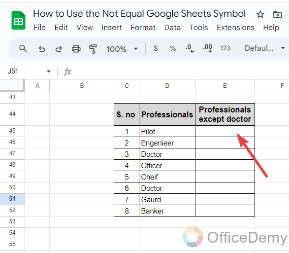
In the following table, we have a list of some professionals for which we need to eliminate “Doctors” only. Let’s see how we can find it with the Not Equal symbol in Google Sheets.

Step 2

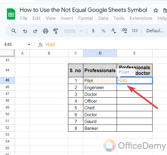
First, we will write the cell address of the data value with an equal sign to run the formula as I have written in the following picture.

Step 3

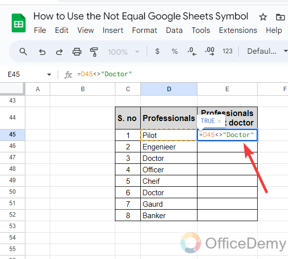
After writing the cell address of the data value, we will use here Not Equal symbol (<>) and then will specify the criteria that is “Doctor” in the following example.

Step 4

When you press the Enter key and drag the formula over the whole list, you will get the following result below. The cells that are not equal to “Doctor” have the result “True” in the cell and the cells containing “Doctor” are indicated as “False“.

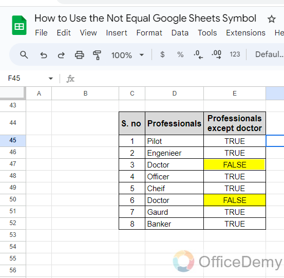
In this way, you can characterize the data by using the Not Equal symbol in Google Sheets.

2. Use the Not Equal with the IF function

As we know, the IF function of Google Sheets is a conditional test or comparison of the values that return a value as true or false. You may also need to make conditions while applying the IF function in Google Sheets. Below is an example of using the Not Equal symbol with the If function of Google Sheets.

Step 1

In this example, we will find the eligibility criteria for the bonus if the cell exists with the help of using the Not Equal symbol in Google Sheets.

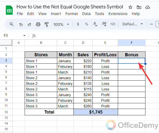
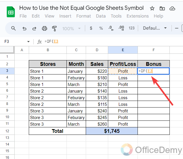
Step 2

First, we will run the “IF” function by just writing IF with an equal sign, after starting the function, we will give the address of the data value on which we are applying the condition.

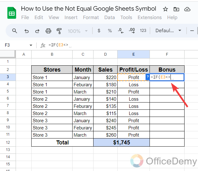
Step 3

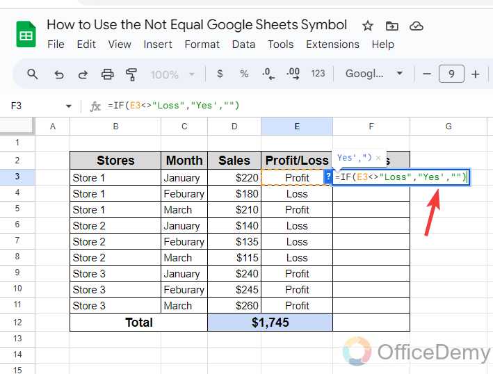
After writing the cell address of the data value, we will specify the criteria according to which we are looking for where we are using “<>” as written in the following picture.

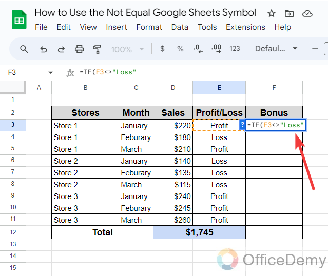
Step 4

Here we will specify that the cell that is not equal to loss for which we will write the syntax in the following pattern. The expression value must be in quotation marks.

Step 5

According to the IF function, after specifying the criteria, we will have to give the values that we will get in return if the value is true or false. Here we will use “Yes” for the value if true and will remain empty if the value is false.

Step 6

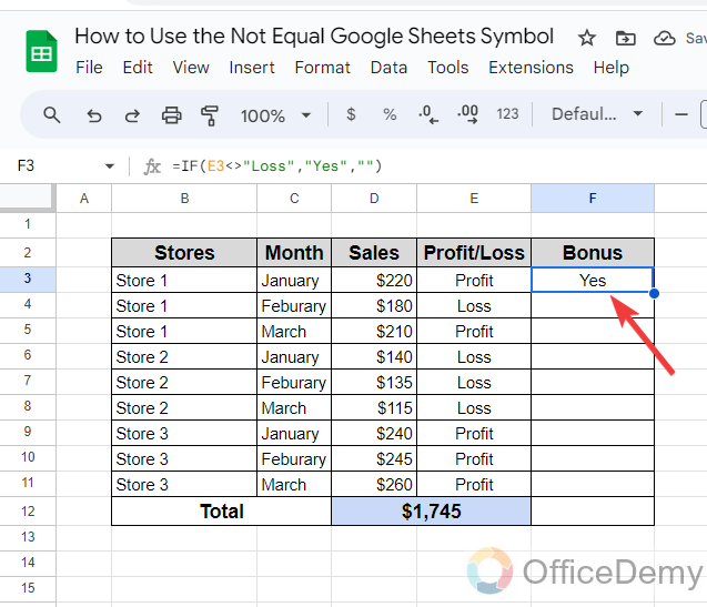
After completing the formula, just press the Enter key to get the result as you can see in the following picture. Now drag this formula over the other cell to see all the results.

Step 7

As you can see in the following picture the cells that do not contain “Loss” have been eligible for a bonus and the rest of the cells are empty.

In this way, we can use the Not Equal sign with the IF function of Google Sheets.

3. Use the Not Equal with FILTER function

Filtering data in Google Sheets is the most essential and useful tool especially when working on a huge list or large amount of data. If you are using the Filter function of Google Sheets to filter data, you may need to use the Not Equal symbol while giving criteria. Let’s not make it too complicated, look at the following example, through which we can see how we can benefit while filtering data using the Not Equal symbol in Google Sheets.

Step 1

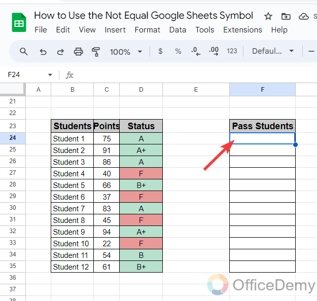
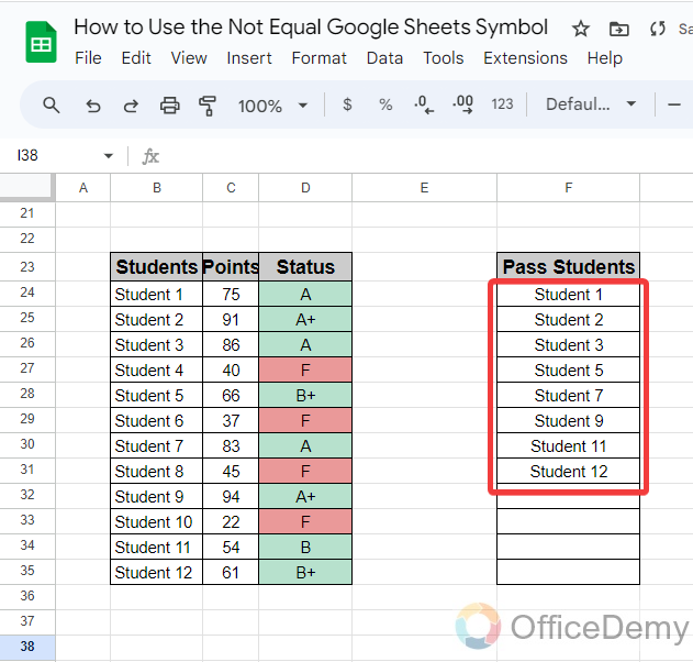
In the following example, we have a table of students with their academic results, while on the other hand, we need to find all the passing students. Let’s see how we can filter it with a Not Equal sign.

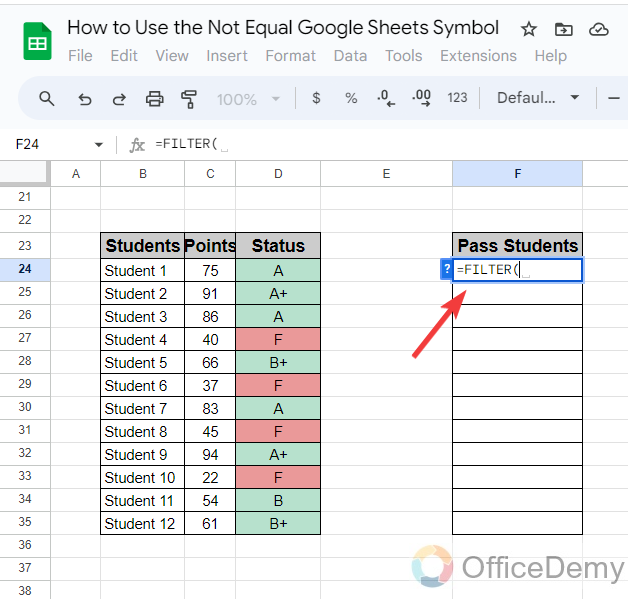
Step 2

Run the filter function of Google Sheets by just writing the “Filter” with an equal sign in the cell as I have written in the following picture.

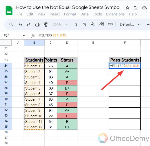
Step 3

First, we will give the data range of the cells that we have to filter, in the following picture we are filtering students, so I have provided the data range of students.

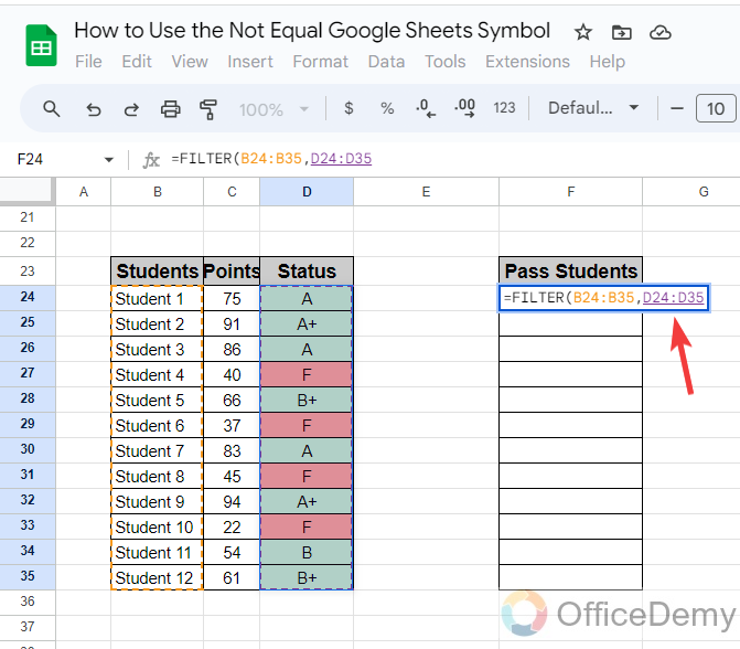
Step 4

After giving the data range, we will have to provide the criteria according to which we have to filter the data. In the following example criteria, the range is the column of results for students.

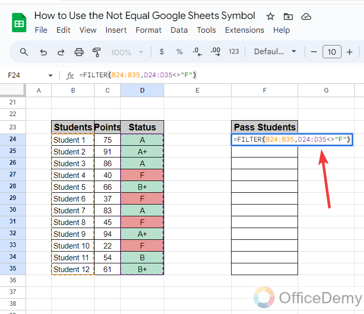
Step 5

We are looking for passing students so, I have written “<>F” in the following picture. It will eliminate all the students who fail and will filter only passing students. Let’s see the result by just pressing the Enter key.

Step 6

Here you can see the result in the following picture, we have gotten the list of passing students as highlighted below.

Frequently Asked Questions

Can I Use the Not Equal Symbol in Combination with AVERAGEIF in Google Sheets?

Yes, you can definitely use the not equal symbol when employing the AVERAGEIF function in Google Sheets. By utilizing the <> symbol alongside AVERAGEIF, you can easily exclude specific values from being averaged in your sheet. This powerful combination offers great flexibility in data analysis when using averageif in google sheets.

How to use the Not Equal with Conditional formatting in Google Sheets?

There are many scenarios where we need to use Conditional formatting like highlighting cells conditionally. These formatting are made by making formula rules where you may need to use the Not Equal symbol in Google Sheets. In the following step-by-step guide, we will show you how you can use the Not Equal symbol in Google Sheets while applying Conditional formatting.

Step 1

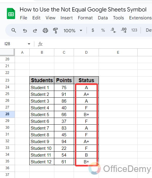
Let’s suppose we have a list of students with their grades. Here we will apply the conditional formatting by using the Not Equal symbol in Google Sheets.

Step 2

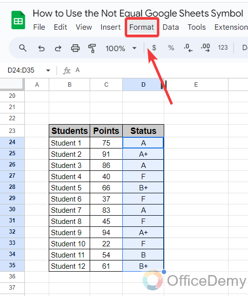
To apply Conditional formatting, the first thing you will need to do is to select the range where we have to apply the conditional formatting, after selecting the range click on the “Format” tab from the menu bar of Google Sheets.

Step 3

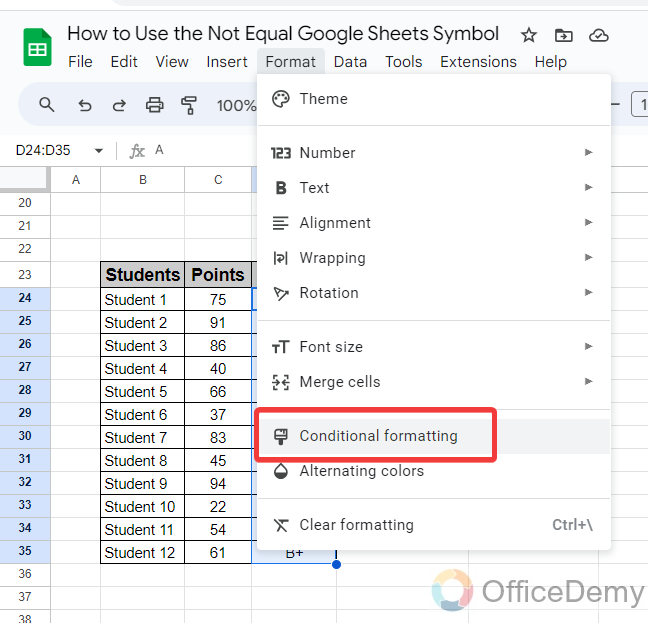
When you click on the “Format” tab, a drop-down menu will open, where you will find the “Conditional formatting” option. Click on it to open.

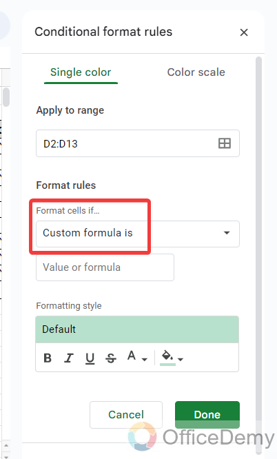
Step 4

When you click on the “Conditional formatting” option, a pane menu will open on the right side of the window. On this page, the menu selects “Format rules” as “Custom formula is” as highlighted below.

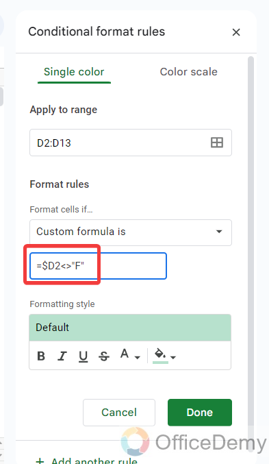
Step 5

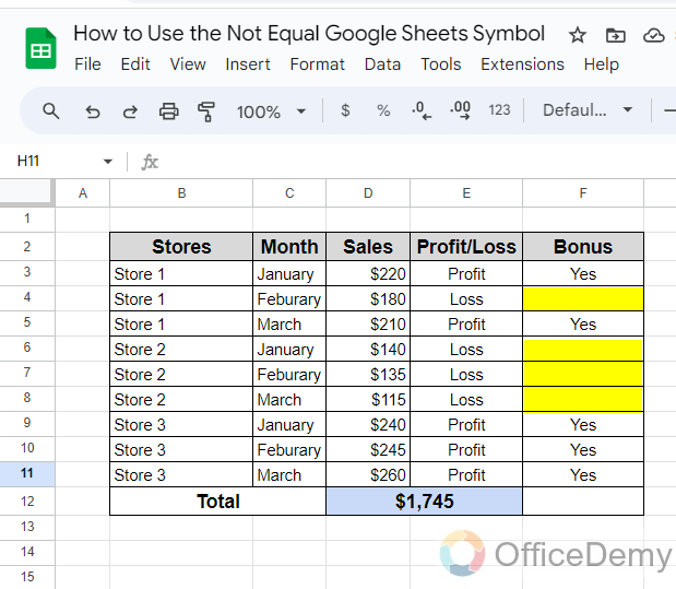
After selecting the rule, we will write the formula “=$D2<>”F” in the formula box, to specify the cells that are not equal to “F“. Now, select the formation, here I am just highlighting the green color in the following example.

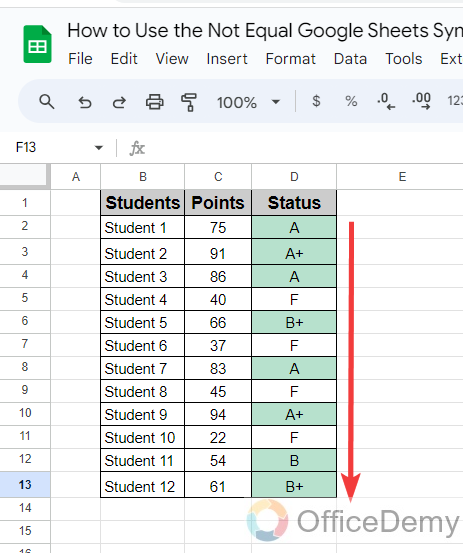
Step 6

The result will be as you can see below, all students who pass have been highlighted with the help of using the Not Equal symbol in Google Sheets.

Conclusion

It is more important to learn when to use the Not Equal symbol in Google Sheets, so we have covered several examples in front of you in the above tutorial on how to use the Not Equal Google Sheets symbol. Hopefully, now, you have understood the logic behind this operation to make your work easy.