
To Use Slicer in Google Sheets
- Import your sample data.
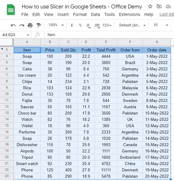
- Select the data range.
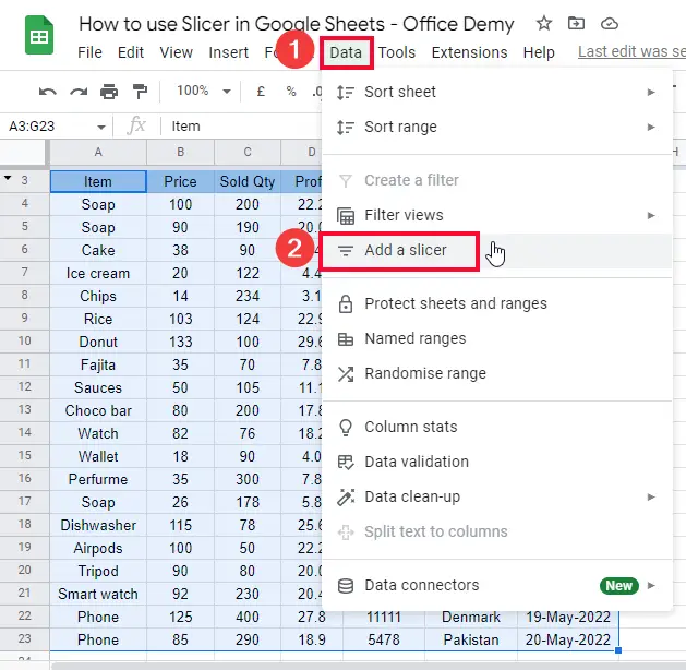
- Go to “Data” and choose “Add a Slicer“.
- A visual slicer will be added to your sheet.
OR
- Double-click on the slicer to open the slicer menu.
- Select a column to filter.
- Use the slicer to filter data visually by selecting specific entities or applying conditions.
Hi, in this article we will learn how to use slicer in google sheets.
What is a slicer? A slicer is nothing but a built-in function that can filter data by a condition or value. It’s not a function like the Filter function, instead, it’s something like a button/dropdown list. Slicer works like a button that can be used visually to filter out data and it helps us o break down a large data set to visually get useful insights into the data set.
A slicer is a visual element, it can be moved freely in the sheet, which means that it’s not inside a cell or range it’s an open-end element that looks like a button. We can use it to draw excellent and useful insights into our data visualized by different column names.
Use Cases of Slicer in Google Sheets
We use the filter function to filter the data based on a condition or multiple conditions and it collapses or expands our data based on the condition, but the filter is a pure function, it is not a visual element. Here, the slicer is fully a visual element, there is no formula or condition, or cell address we need while using the slicer. Slicer is like a button we can move it around the sheet and customize it very beautifully using font size, colors, background color, text size, and many other editing features.
A slicer works like a filter, it can filter data by a condition or by values. We need to learn it to draw valuable insights of the data, let’s say you have data of items sales of the month, now you want to see the top selling items, you can easily use a slicer to it, slicer can also be connected with pivot tables and charts to make a dashboard. On the other hand, filters cannot be used like that, they do not give us a visual representation of the filtered data they just collapse the data and show only the filtered data values. We need to learn how to use slicers in google sheets to see how it helps us make useful visual insights of the data based on conditions or values.
How to use Slicer in Google Sheets
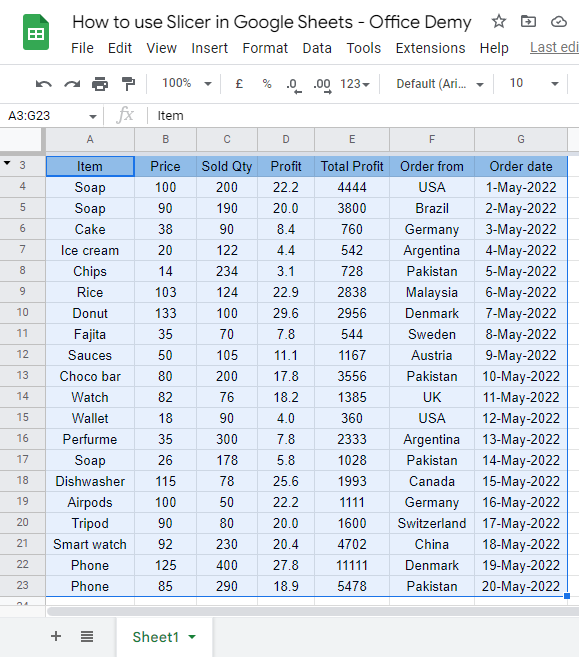
Here, we will see everything related to the slicer. We will see various methods and procedures to add and use slicers with our data. For this tutorial, I have a dummy data set that shows the product sales data for the previous months. Let’s see how to go with it and use slicer in google sheets.
How to use Slicer in Google Sheets – Adding a Simple Slicer
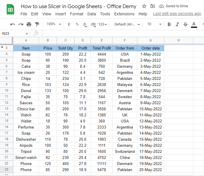
Adding a slicer in google sheets, we need some sample data.
Step 1
Sample data
Step 2
Select all data
Step 3
Go to Data > Add a Slicer
Step 4
A visual slicer will be added to your file.
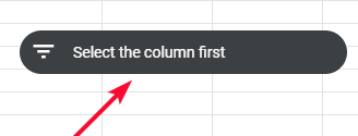
Note: This slicer will do nothing in this state. So, we need to set up the slicer to make it useful.
How to use Slicer in Google Sheets – Filter data using Slicer
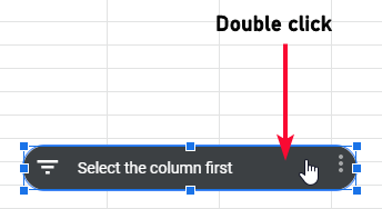
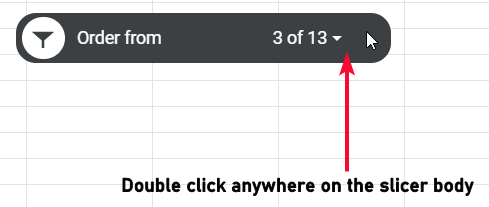
To set up the slicer we need to double-click on it to open the slicer menu on the right-hand side.
Step 1
Double click on the slicer
Step 2
Select a column
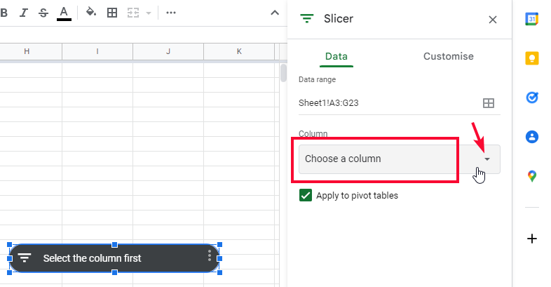
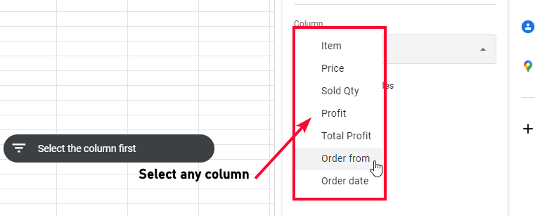
Note: A slicer can take only one column at once.
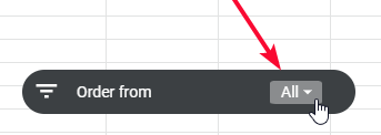
Step 3
Now you can use this slicer to filter your data visually, click on the “All” dropdown, and select the entities from your selected column to filter out the data.
Step 4
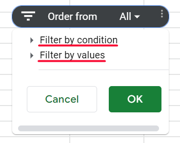
Now we can use “Filter by condition”, or “Filter by values”
Step 5
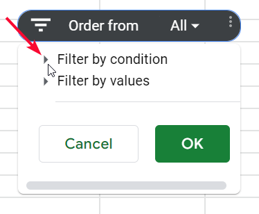
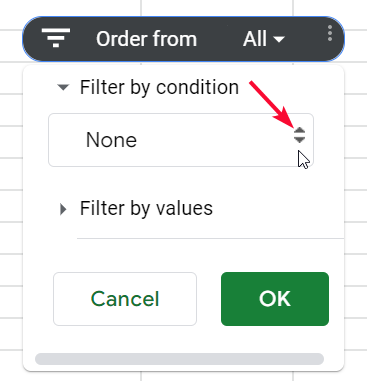
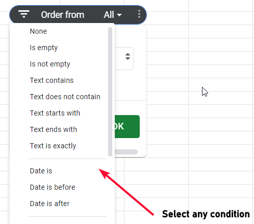
Click on “Filter by condition” and select a condition from the drop-down (similar to conditional formatting)
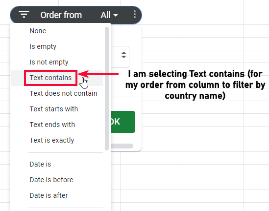
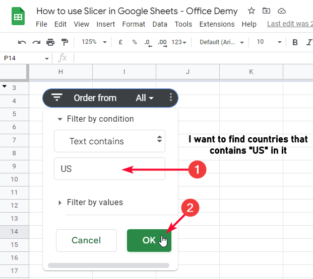
Step 6
Define the condition, and click on OK
Step 7
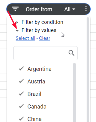
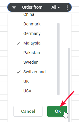
Click on “Filter by values” and select from the values, it’s more like a manual method.
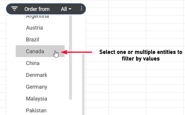
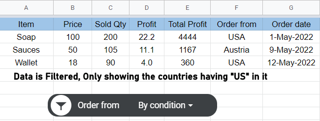
Step 8
As you click on Ok, the data will be filtered and collapsed
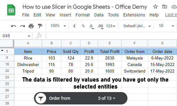
This is how you can filter your data using Slicer, and this is how to use slicer in google sheets.
How to use Slicer in Google Sheets – Customizing the Slicer
In this section, we will quickly learn how to use the slicer in google sheets and how to customize the slicer, by color, font size, background color, title, etc.
Step 1
Double click on Slicer, Slicer editor will open on the right-hand side
Step 2
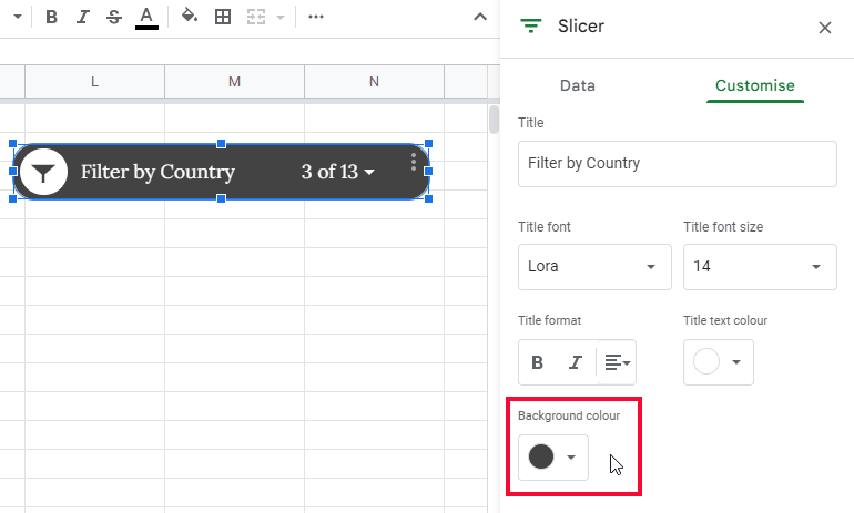
Go to Customize tab
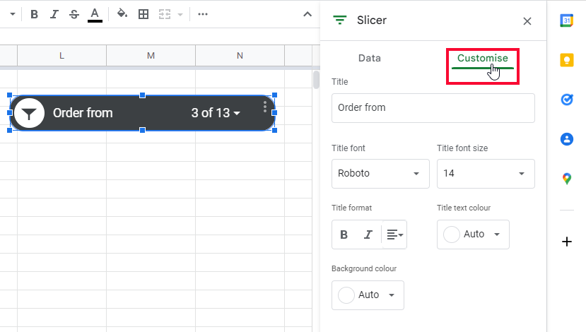
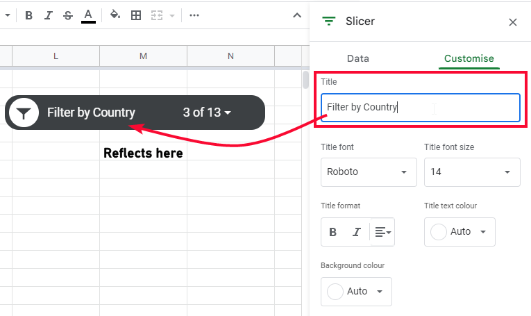
Step 3
Here you can change the title of the slicer and give it a meaningful name.
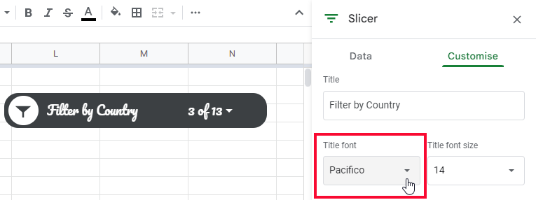
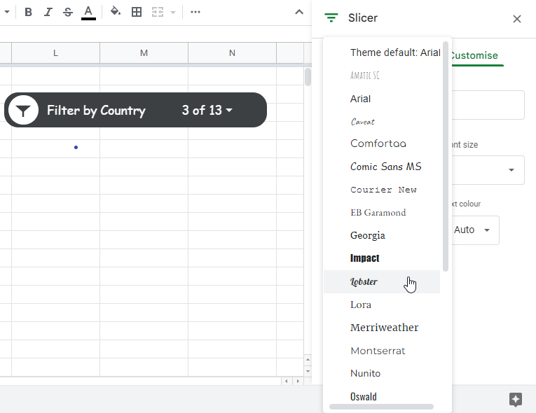
Step 4
You can change the title font family
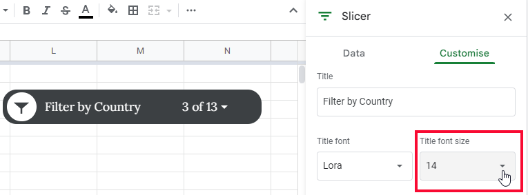
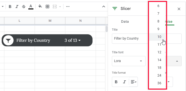
Step 5
Next, you can change the font size of the title
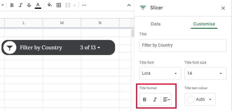
Step 6
Below, you can use “bold” or “italic”, and you can set the text alignment as well
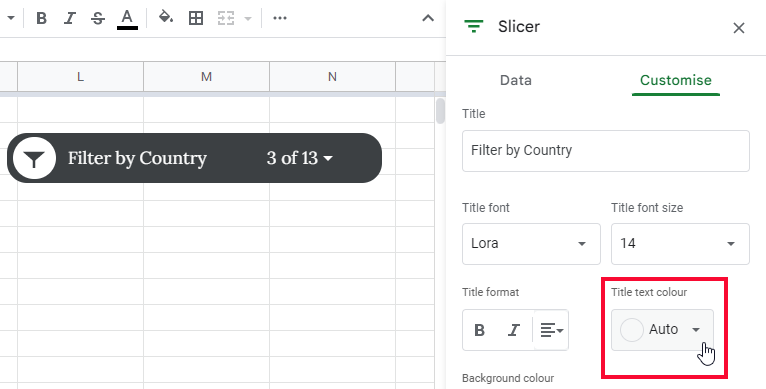
Step 7
Next, you can set the title text color
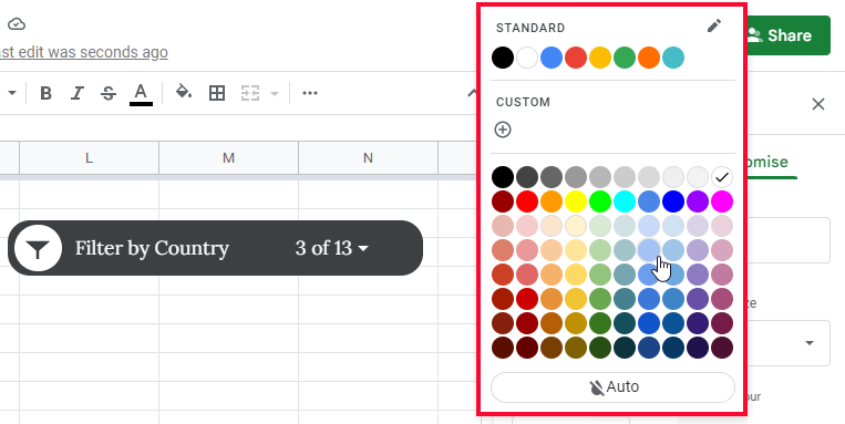
Step 8
Finally, you can set the background color of the slicer

This is how you can customize your slicers, there are some more options to see that come with slicers.
Click on the three dots on the right top of the slicer
Here,
Edit Slicer: opens the slicer menu (identical to double clicking on the slicer)
Copy Slicer: copy the slicer into the clipboard
Delete Slicer: deletes the slicer
Set the current filter as default: set the current filter as the default filter
Learn more: will open the help window
How to use Slicer in Google Sheets – With Pivot Table
Pivot tables are more useful when working with slicers, we can make and use pivot tables of our original data and can work with Slicers, it helps us more to minimize the data and keep only the useful data in the pivot table. Let’s see how we quickly make a pivot table and work with slicers
Step 1
Select all the data
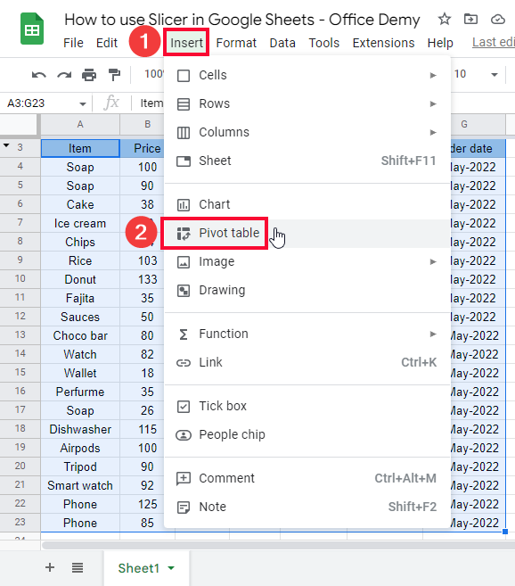
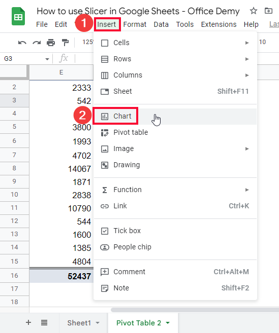
Step 2
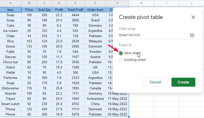
Go to Insert > Pivot Table
Step 3
Select New sheet (only for keeping things organized and clean)
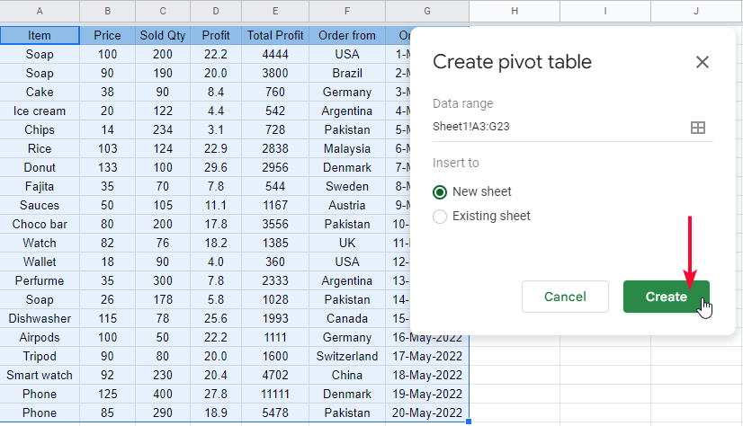
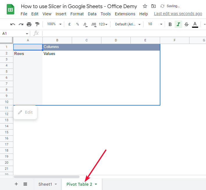
Step 4
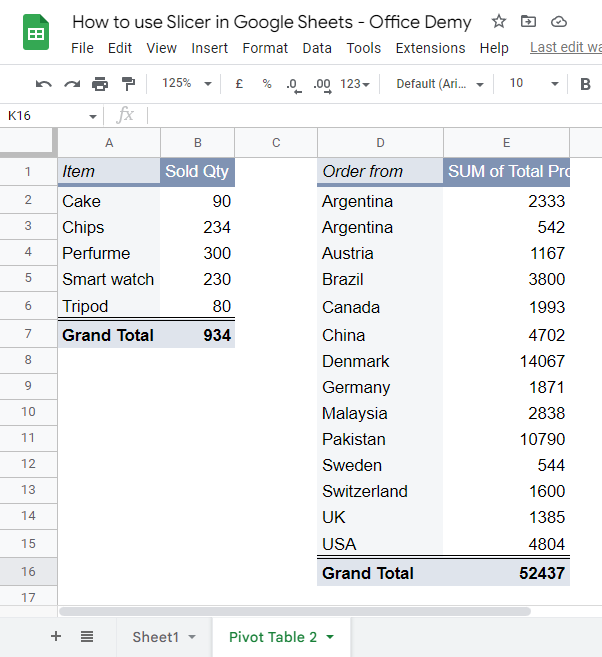
Click on create, and a pivot table will be created on a newly created sheet into the same workbook
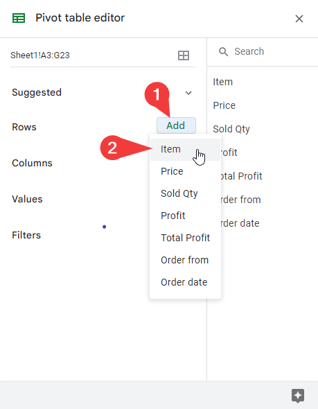
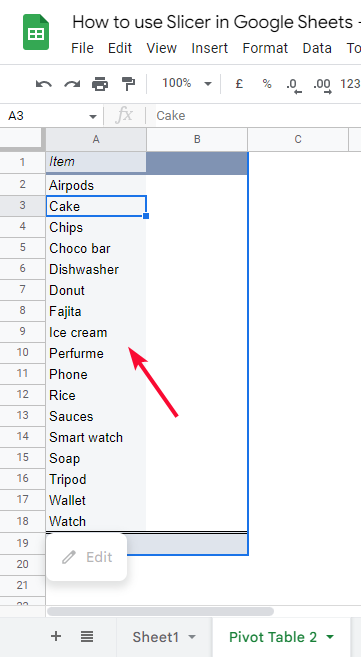
Step 5
In the pivot table editor, add a row by clicking on the add button (you can add any row, here I am adding the products)
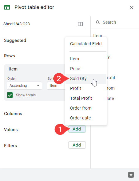
Step 6
in the next column, click on add in the Values section to add values in this column (select any column for, I have selected sold Qty)
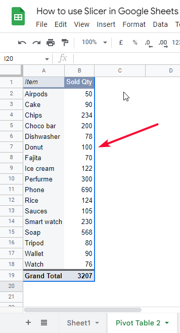
Step 7
Now you have a simple summary of your data, you can add a slicer and the data inside the pivot table will be filtered as you specify it using the slicer.
This is how you can work with pivot tables and slicers.
How to use Slicer in Google Sheets – Creating a Mini Dashboard
We can make a dashboard using a pivot table, slicer, and charts. In this section, we will see how to use a slicer in google sheets to create a dashboard. For this, we need to make a chart, and also, we can make more pivot tables (optional)
I am using a pivot table and chart to make a dashboard; I will also create multiple slicers for multiple columns of my data.
Step 1
Create the pivot tables, you can create as much as you need (as we created in the previous section)
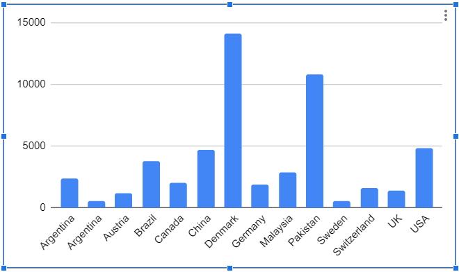
Step 2
Create a column chart, with the pivot table’s data (or you can add any chart as per your preferences)
Step 3
Add some slicers (use source data, not the pivot table’s data) and assign a different column to each (use the source data for the slicer)
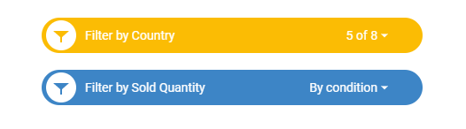
Step 4
Now you can use various filters and you can see the real-time changes in the pivot table and the chart.
This is how you can use the combination of slicers, pivot tables, and charts to make an amazing dashboard for your datasets.
Get How to Use Slicer in Google Sheets Free Template
Note: Make a copy and work on the copy, do not ask for editor’s access.
Useful Notes on How to use Slicer in Google Sheets
- Slicers can have only one column at once
- Slicers can be resized freely
- Slicers can be customized
- Slicers are visual elements that look like a button and work like drop-down filters
Frequently Asked Question
Can the Slicer tool be used to slice strings in Google Sheets?
Yes, the Slicer tool in Google Sheets allows for efficient google sheets string slicing. This feature enables users to quickly extract sections of text from a string and organize the data accordingly. By selecting the desired slicing range, users can manipulate and analyze strings in a more precise and effective manner.
How slicers are different from filters?
There are many differences between slicers and filters to talk about, but the primary difference is the difference between the visual representation and the imperceptible view. This makes slicers more accurate to use when making dashboards like presentations in google sheets. We can filter out data based on conditions or values. Another major difference is slicer is not a function or formula we don’t need to deal with the syntax, whereas the filter is a pure function that follows a syntax. Slicers can be freely moved, resize, customized, and can show data visually very easily. These are the main differences between slicers and filters.
Conclusion
Wrapping up how to use Slicer in google sheets, we have learned about the slicer, how it works, and why they are so helpful in the visualization of the data in google sheets. In this tutorial, we have covered several things like pivot tables, slicers, and also charts. We have seen how to use the combination of these three features of google sheets to make excellent dashboards. We have learned how to make a simple slicer, how to set up a slicer by assigning a column, and how the is filtered based on conditions and values in the slicer. We then discussed the customization of the slicer, and have seen several editing options we have in the slicer editor. We also saw how to make pivot tables to work on summarized data with slicers, and then finally we created a dashboard, and using various slicers we made a dashboard with several columns of data using multiple slicers. I hope you find this article helpful and that you have learned many new things. Don’t forget to like share and subscribe to Office Demy for more exciting updates. Thank you so much. Keep learning with Office Demy.


