The FLATTEN Function in Google Sheets – User Guide

Hi, in this guide, we will learn how to use the FLATTEN function in Google Sheets. However, the Flatten is an uncommon function of Google Sheets but still, it is a very useful function in Google Sheets. The flatten function of Google Sheets is to flatten the data into a single column. If you have a data set consisting of multiple columns and rows but you want to convert this data into a single column, then you don’t need to write down it again manually. Fortunately, there is a built-in function in Google Sheets that can flatten your data into a single column in Google Sheets. In this tutorial on the flatten function in Google Sheets, we will teach you multiple examples of how you can flatten data in Google Sheets.

Benefits of the FLATTEN Function in Google Sheets

The Flatten function of Google Sheets is a powerful tool of Google Sheets that can help you to convert multiple columns of data into a single column in Google Sheets. Flatten function can be very useful too when you need to combine any data into a single column. You can also arrange multiple columns into a single column individually with the help of the flatten function in Google Sheets. Let me show you practically all these actions done by flatten function in the following section.

Step-by-step Procedure – The FLATTEN Function in Google Sheets

The usage of the Flatten function is very fine and easy because there is only a single argument in the syntax of the Flatten function of Google Sheets. In this tutorial on the flatten function in Google Sheets, we will go through the several different uses of the Flatten function to understand the anatomy of the Flatten function. So, let’s get started without wasting our time.

Example # 1: Simple use of the Flatten function

In this example of the flatten function, we will apply the flatten function of Google Sheets on a simple data range to flatten data into a single column.

Step 1

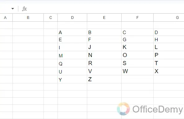
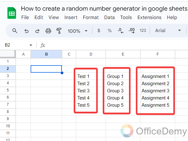
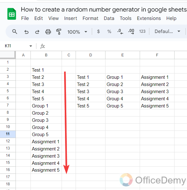
Let’s suppose, you have multiple ranges of data in Sheets or such type of data with different rows and columns as can be seen in the following picture, and want to shift in one single column. Let’s see how we can flatten data with the help of the flatten function in Google Sheets.

Step 2

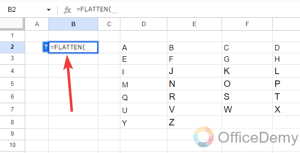
First, select the column or cell where you want to flatten your data place the cursor in it, and start the flatten function of Google Sheets by just writing Flatten with an equal sign.

Step 3

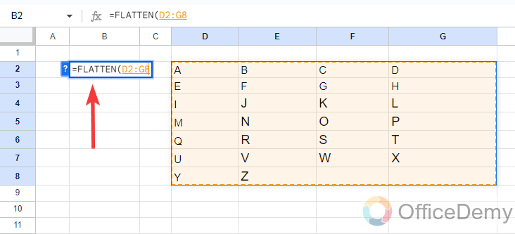
Once you have started the flatten function, there is only a single argument in the flatten function of Google Sheets which is range. Provide the data range that you want to flatten as I have given in the following screenshot.

Step 4

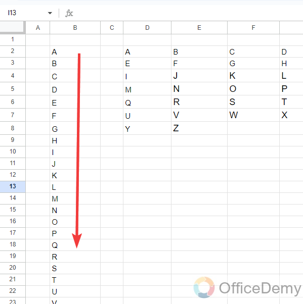
There is nothing more to do, just press the Enter key after giving the data range into the syntax, and your all data will be set into a single column as you can see the result in the following example.

Example # 2: Labels by Flatten Function

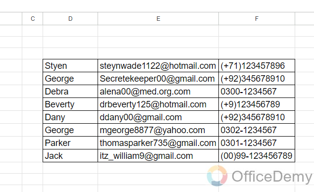
If you have basic personal information in multiple columns like (Names, addresses, emails, and phones) you can also create a pattern of labels in Google Sheets by using the flatten function. Let me show you practically in the following guide.

Step 1

Here, we have names in the first column, addresses in the second column, and phone numbers in the last column. Now, let’s see how we can arrange them all into a single column to make label data into Sheets by using the flatten function in Google Sheets.

Step 2

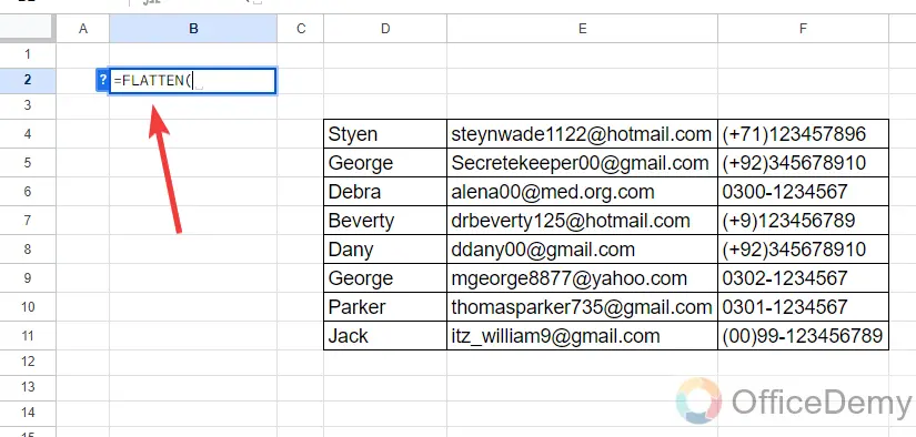
First, simply start the flatten function of Google Sheets in the cell where you want to flatten your data range as directed below.

Step 3

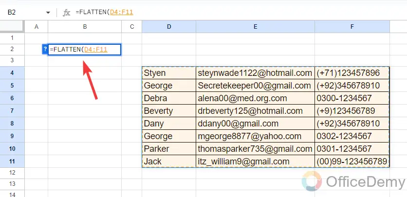
After starting the flatten function into the cell, provide the data range that you want to flatten as I have given in the following example.

Step 4

There is only a single argument in the flatten function, once you have given the data range then just simply press the Enter key, as you press the Enter key, your all data will be flattened in the following way as directed below.

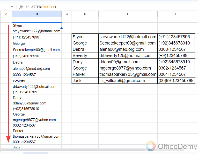
You can use this data as a label for an envelope or any other template. 

Example # 3: Flatten function for individual ranges

The Flatten function of Google Sheets flattens the data horizontally across all ranges but if you want to flatten your columns individually in vertical division then you will have to follow the following instructions that are described below.

Step 1

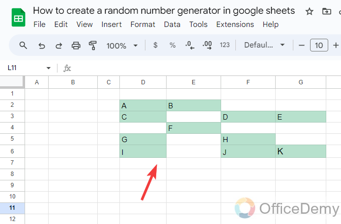
In the following sample data, we have 3 different columns that we want to flatten individually. Let’s see how we can do that with the help of flatten function in Google Sheets.

Step 2

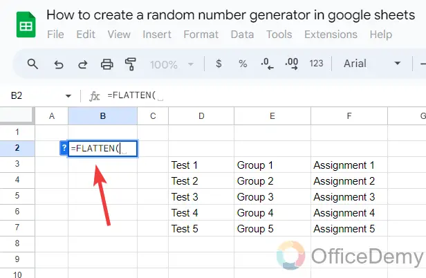
As above, first, start the flatten function in the cell where you want to flatten your data in Google Sheets by just writing Flatten with an equal sign.

Step 3

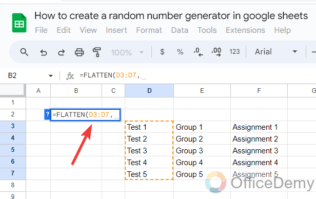
After starting the flatten function, give the range of the first column only as I have written in the following picture, and then add a comma sign.

Step 4

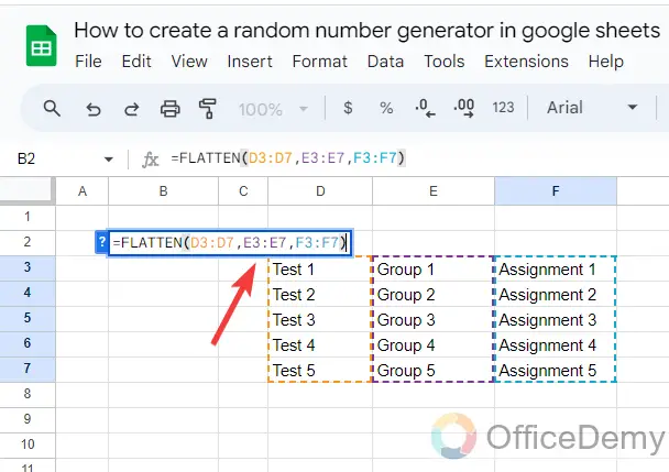
After giving the range of the first column, similarly, specify the range of the second column and third column respectively. These ranges are separated by a comma sign as directed below.

Step 5

After giving all ranges just close the bracket and press the Enter key to get the result as I have gotten in the following example. Here you can see in the flattened data, that there is first column data, second column data, and then third column data as required.

The FLATTEN Function in Google Sheets – FAQs

Q: How to flatten data in an array in Google Sheets?

A: Let’s suppose, you have irregular data in multiple columns and rows that you want to flatten, it will also give you the irregular results in flattening data. In such a situation, how to flatten data in an array in Google Sheets. Let me show you practically with the help of following instructions with an example.

Step 1

In the following sample data, you see that we have several values in different ranges with some empty cells. Let’s see what we will get when we flatten this data in Google Sheets.

Step 2

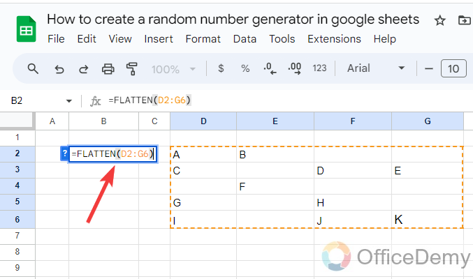
Here, first, we will start the flatten function in the cell, where we want to flatten the given data, and then will provide the whole range that includes values in it as highlighted in the following picture.

Step 3

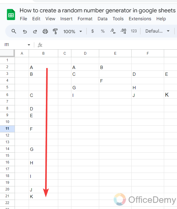
Now, once you have given the range, as you press the Enter key, you will see that your data has been flattened but also included with those empty cells that were in the dataset. Now, let’s see how we can flatten this type of irregular data into an array.

Step 4

Hover your cursor over the formula cell and make it editable add the “UNIQUE” function in the syntax after the equal sign and add small brackets at the beginning and end of the syntax.

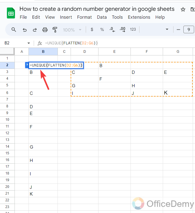
Step 5

Now, if you press the Enter key, you will get all your data flattened into an array as can be seen in the following picture.

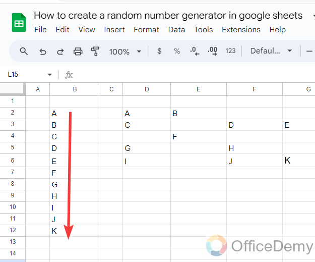
In this simple way, you can flatten any irregular data into an array in Google Sheets.

Q: Can we unpivot the flattened data in Google Sheets?

A: Yes! If you want to remove the flattened data then simply remove the flattened syntax from the cell, you all flattened data will vanish but if you want to unpivot the flattened data into the Google Sheets then you will have to use the following formula to unpivot the flatten data in Google Sheets.

=ArrayFormula(SPLIT(FLATTEN(first_column_range&”❄️”&first_row_range&”❄️”&data_range),”❄️”))

Conclusion

Many users didn’t know about the flatten function in Google Sheets, hope with the help of the above guide you all know about the flatten function of Google Sheets and can use it in your spreadsheet tasks.