How to Use Rank in Google Sheets [Top Guide]

Hi, today we will learn how to use Rank in Google Sheets. There are so many built-in functions in Google Sheets used to perform automatic calculations and solve conditions. The Rank is one of the powerful tools of Google Sheets that is used to analyze and sort data to make informed decisions on rankings. If you are not aware of this function tool of the Google Sheets then go through the following article on how to use Rank in Google Sheets in which we will take a deep overview of using the RANK function. So, let’s get started.

Why do we need to use rank in Google Sheets?

The RANK function is essential for the analysis of a balance sheet mostly because it has the capability of identifying the relative performance of different items within a balance sheet.

By ranking these items, you can easily find data inclined, trends, and potential areas of relative values. The rank function can be also used to provide information that can be invaluable for making informed financial decisions and evaluating the overall financial health of a company.

You can also use the rank function to determine the final results of different marksheets etc.

How to use Rank in Google Sheets

The rank function in Google Sheets is used differently in different scenarios. If you want to rank the data in ascending order, the syntax will be different, if you need to rank the data in descending order, the syntax will be different and if you want to find the rank of a number in arrays then the syntax will be different. Let’s see all of these scenarios with the help step-by-step guide below.

1. Rank the data in ascending order
2. Rank the data in descending order
3. Rank data with arrays

Rank the data in ascending order

Let’s suppose you have the data of some students with their points and you want to rank them with highest to lowest mark or in ascending order then use the following method.

Step 1

First, make a separate column beside the data that you want to rank and then place your cursor in it.

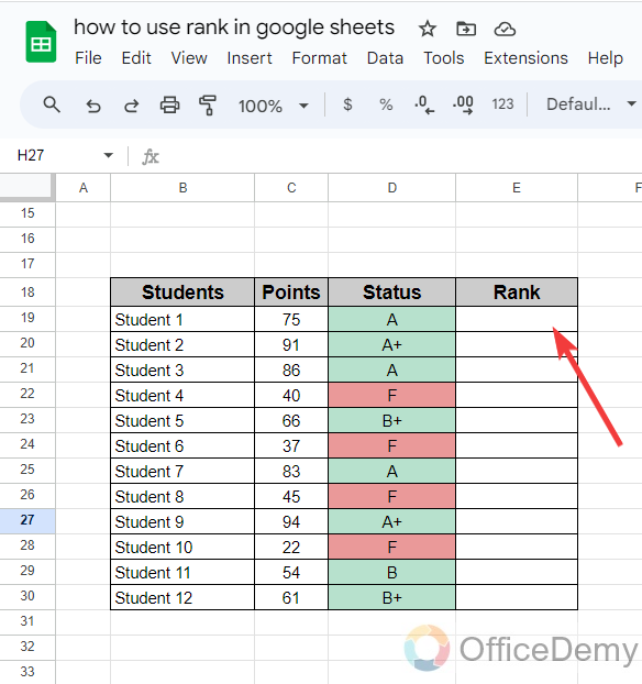
Step 2

Run the RANK function by simply writing the “Rank” with an equal sign as I have written below.

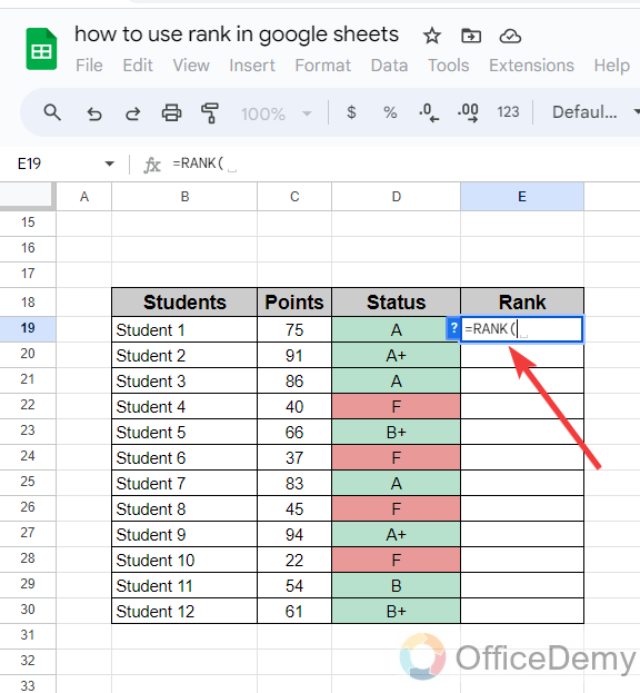
Step 3

After starting the RANK function, first give the value that we want to rank from the data in the following example we want to rank the students with their points so we have given the cell reference of the student’s points.

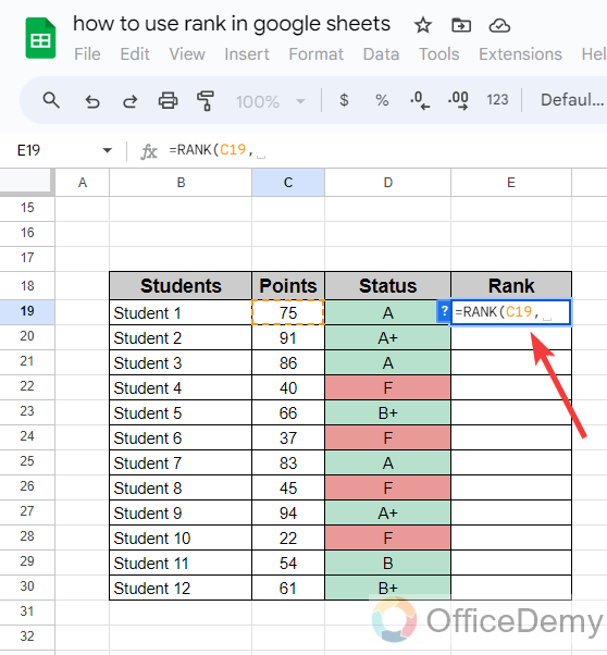
Step 4

After giving the value in the RANK syntax the second argument will be the data in which we are ranking the number that is the entire data range of Students points in the following example.

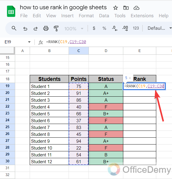
Step 5

The third and the last argument in the syntax of the RANK function is False or True which indicates whether it is ascending or descending. In the following example, as we are ranking the data in ascending order we will write “False” for ascending order.

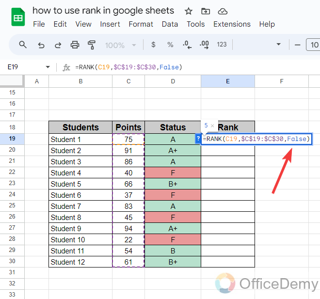
Step 6

We have completed the syntax, we will get the result as we press the Enter key. You will find the rank of a given number in the specified data, If you want to see all the ranks then drag down the formula or you can click on “Autofill“.

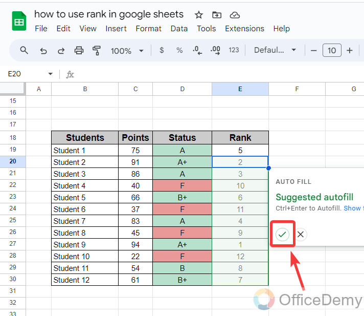
Step 7

Here, you can see the result in the following picture, Your data has been ranked now in ascending order as you can see the highest point is indicated as ranked 1st.

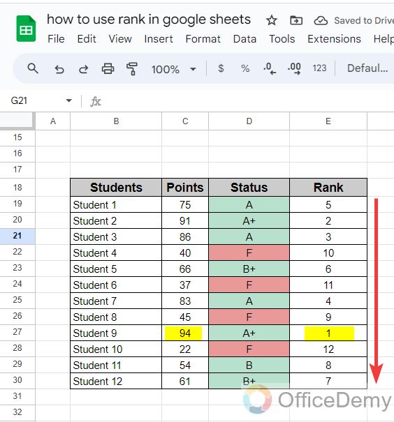
Rank the data in descending order

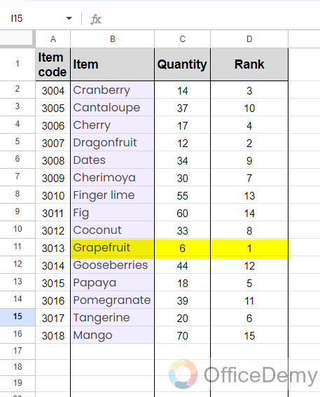
In this example, we will rank the data in descending order. Let’s suppose you have sample data of some items with their quantity and want to look at the least quantity item then the following condition may be helpful.

Step 1

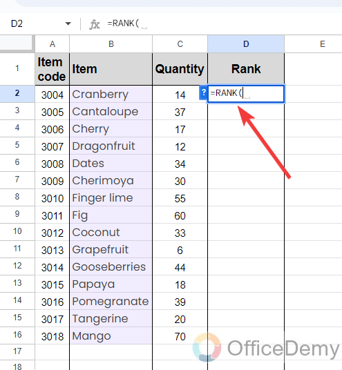
As you can see in the picture, we have a list of items with their quantity, we want to check the stock and which item is ending so we may find it with the rank formula.

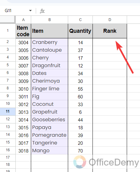
Step 2

Simply, first run the function by writing the “Rank” with an equal sign in the cell where you want to rank the data.

Step 3

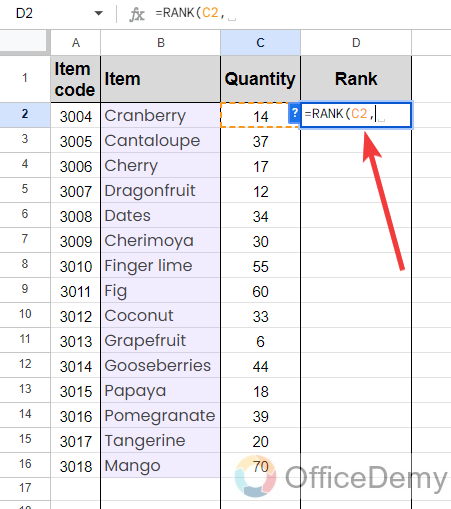
The first argument of the syntax is the value that you want to rank. Here we want to rank the data with the quantity of items so we will give the cell reference of item quantity.

Step 4

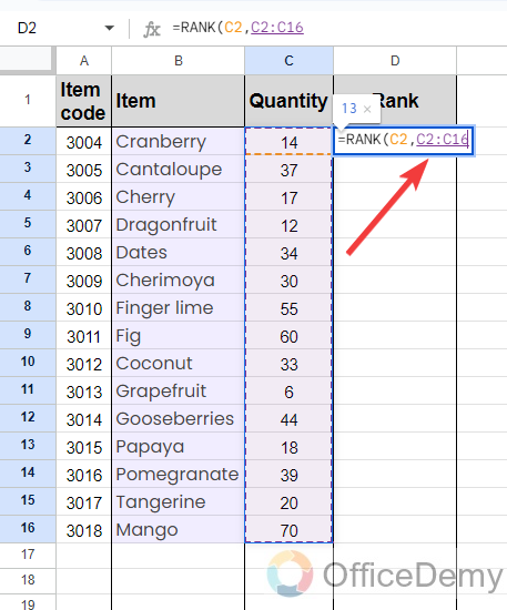
After giving the value in the RANK function syntax, we will have to give the data range in which we are ranking the data that is C2:C16 in the following example.

Step 5

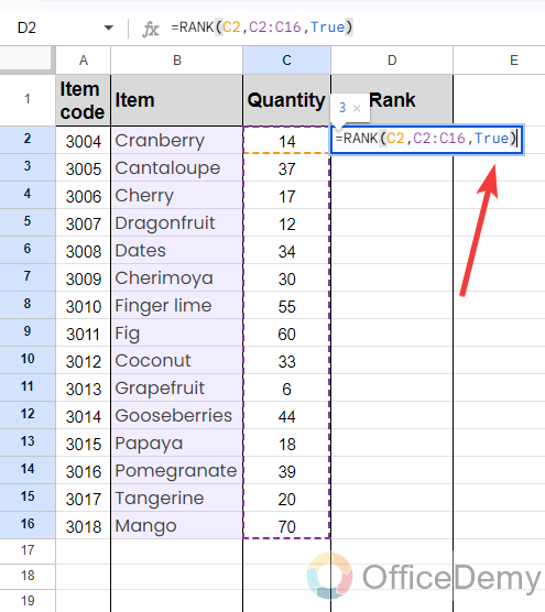
As we are ranking the data in descending order, after writing the data range, we will write the “True” to rank the data in descending order.

Step 6

Pressing the Enter key will give you the result as can be seen in the following picture, the data has been ranked in descending order.

Rank data with arrays

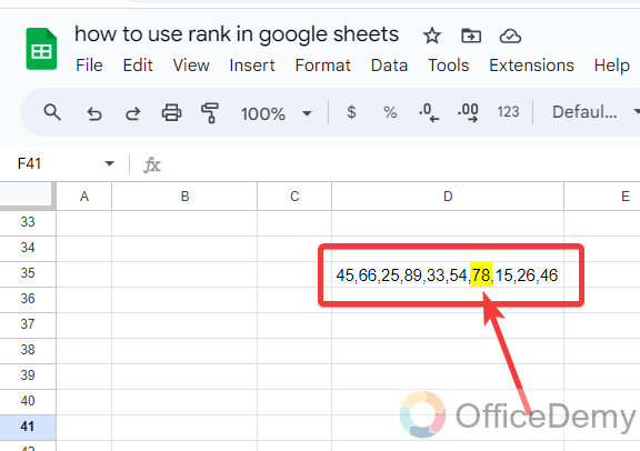
Let’s suppose, if you have a number sequence in which you want to find the rank of any number then you may find it with the Rank function.

Step 1

As you can see in the following example, there is a sequence of different numbers in which I want to find the rank of the number 78.

Step 2

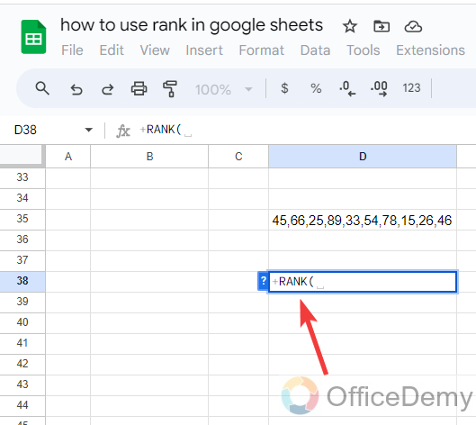
Run the RANK function with an equal sign in the cell where you want to find the rank of the number as I have written below.

Step 3

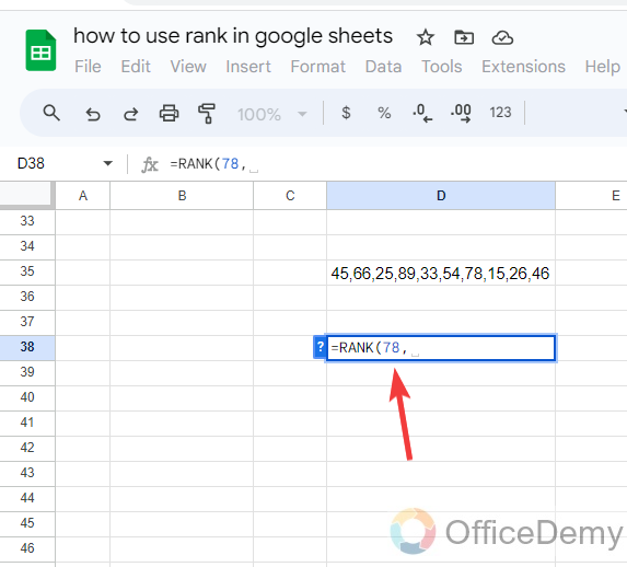
As we know the first argument of the RANK function syntax is the value that we want to rank, so here we will write the number “78” after starting the formula.

Step 4

After giving the value in the syntax, the second argument will be the sequence in which we are looking and this range must be in curly bracket as written below.

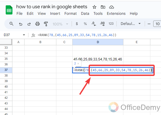
Step 5

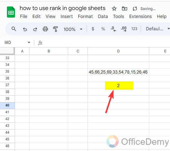
Now, just need to press the Enter key and you will get the result as you can see in the following screenshot, we have got the rank of 78 number in the given sequence of numbers.

Frequently Asked Questions

Is Knowing How to Use Rank in Google Sheets Helpful for Performing a T-Test in Google Sheets?

Knowing how to use rank in Google Sheets can be helpful when performing a t-test in Google Sheets. By using the google sheets test, you can easily identify and order values, enabling you to determine the ranks of specific data points. This functionality can be beneficial when analyzing data sets and conducting statistical tests like the t-test in Google Sheets.

How to see the top five ranks in the Google Sheets?

Let’s suppose, you have a list of items with their quantity, now we have to find the top five least quantities so we may order them to fulfill the stock.

Step 1

Here, first, we will apply the RANK formula in descending order so we may find the rank of the values from least to highest as we have found below.

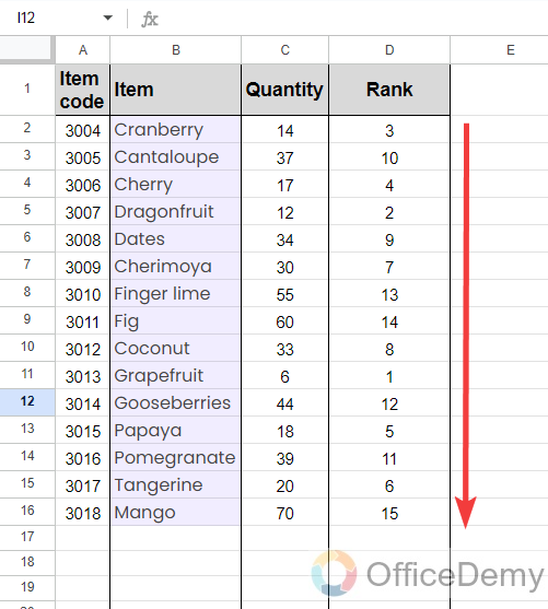
Step 2

But if you have a long list and you are having difficulties finding the top five ranks in the list then simply select all the ranges.

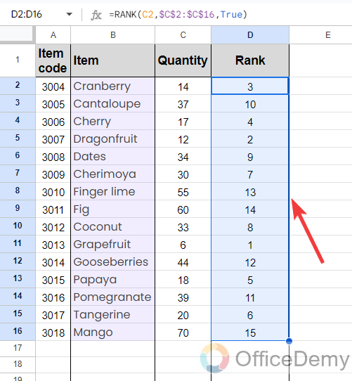
Step 3

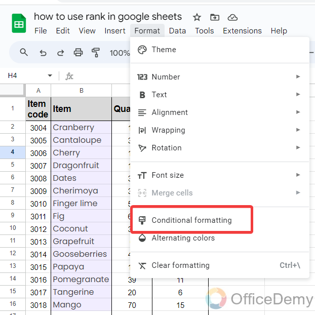
Then go into the “Format” tab from the menu bar of Google Sheets and click on the “Conditional Formatting” option as highlighted below.

Step 4

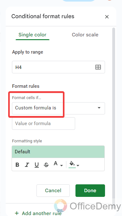
In the Conditional formatting pane menu, select the format rules to “Custom formula is” as highlighted in the following picture.

Step 5

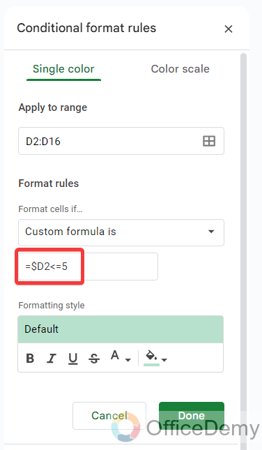
Here, I will give the criteria “=$D2<=5” which means the values less than are equal to 5 in the given cell range.

Where column D is for the ranks of quantities.

Step 6

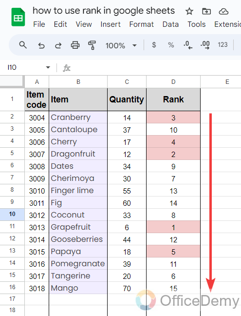
So, it will automatically highlight the top 5 of the ranks as highlighted in the following picture. In this way, you can easily find the top 5 in Google Sheets.

Conclusion

In the above article on how to use rank in Google Sheets, we have learned all the scenarios that are used in the RANK function of Google Sheets, hope now you will not face any trouble using the RANK function in Google Sheets.