How to Calculate Google Sheets Running Total [3 Ways]

Today we will learn how to calculate Google Sheets running total. As we all know Google Sheets has more expert features and functions to make calculations than when it is talked about to calculate the running total in Google Sheets. How can it be behind? Due to flexibility and smooth functioning, calculating the running total in Google Sheets becomes very easy.

In today’s topic, we are going to discuss how to calculate Google Sheets running total. If you also want to know how to calculate the Google Sheets running total, then join us and go through the following guide.

Why do we need to Calculate Google Sheets Running Total?

If you are dealing with a large amount of data including daily expenses, you might want to know the sum of expenses for a few consecutive days at a given time. If you are a cashier and calculate the amount of total purchases made by the customer, then you may need to calculate the running total.

Similarly, it may be used in various scenarios like adding a points table for any game, scoring, budget calculating, reporting, and billing, etc.

How to Calculate Google Sheets Running Total

Calculating the running total in Google Sheets is very simple but it may vary into different categories as per given data. We will learn all of them in the following article and also will discuss the reason behind the use of this method so you may understand the logic of every situation to find a running total in Google Sheets.

1. By simple addition operator
2. By Sum function
3. Dynamic running total

1. Running Total by Simple Addition Operator

This is the most useful and easiest way to calculate the running total because in this method you don’t need to require any function to calculate a running total in Google Sheets, you can find the running total by just performing an additional operation on the values. Let me show you practically in the following steps, how you may calculate the running total by just adding values.

Step 1

If you see in the following example, we have sample data of expenses daily, in the other column, we need to find the “Running total” accordingly.

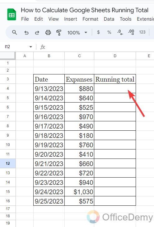
Step 2

First, place your cursor where you want to get the running total in Google Sheets and give the cell address of the first value as I have given below.

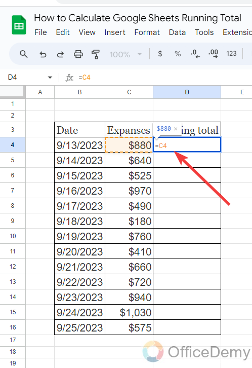
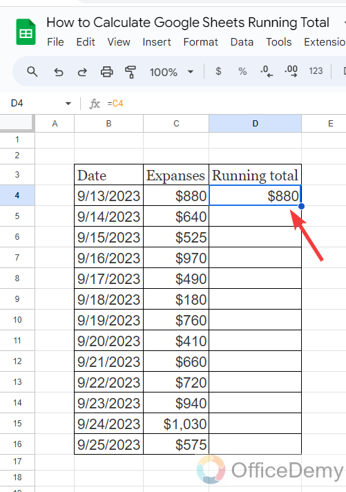
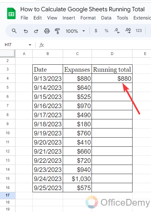
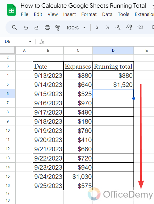
Step 3

After giving the cell reference of the first value, just press the Enter key, and you will get the same value in the first cell of the running total as can be seen in the following picture.

Step 4

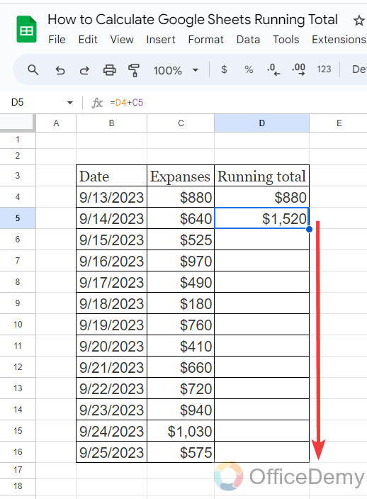
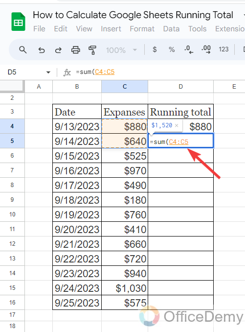
Now, in the second cell of the running total, give the cell reference of the first value of the running total then add this value to the second value of expanses in the following pattern.

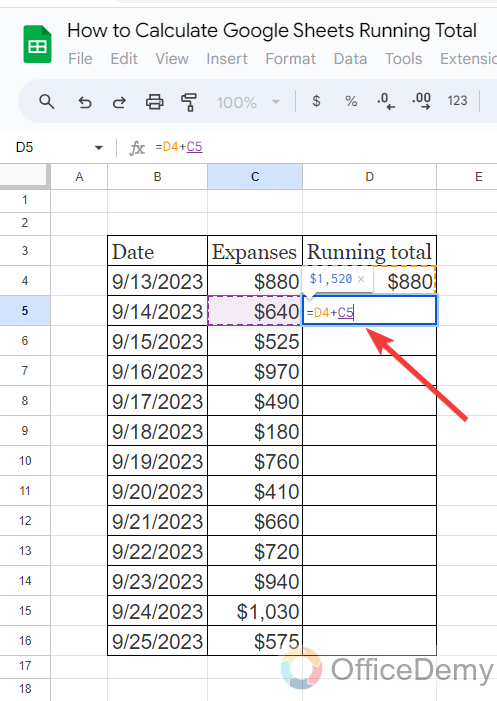
Step 5

As you press the Enter key, you will get the first value of the running total as can be seen below as well. If you want to continue this formula to calculate further values, just drag the formula over the other cells.

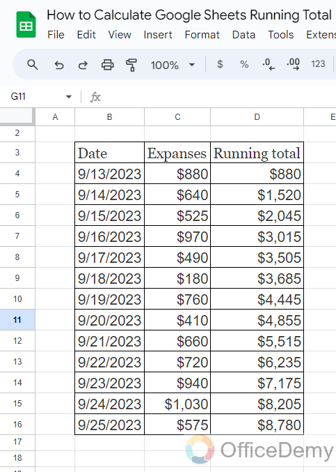
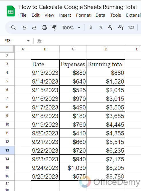
Step 6

The result is in front of you, in this simple way you can calculate the running total in Google Sheets.

2. Running Total by Sum Function

As we have seen in the above method, there is only one operation of adding values in calculating the Google Sheets running total that we can also find by applying the sum function of Google Sheets. The advantage of this method is that you can also array your Google Sheets running total. Go through the following steps to calculate the Google Sheets running total by the Sum function.

Step 1

In this method as well, first, we will write the first value of expenses as it is, as I have written below. This value can be written normally as well or by formula.

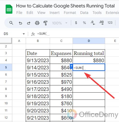
Step 2

Once you have found the first value of running total, then in the second cell start the Sum function by just writing “Sum” with an equal sign.

Step 3

After starting the Sum function, we will give the cell reference of data values of the first and second cells. As here first values are the same, we have written “C4:C5“, where you can also write “D4:C5“.

Step 4

Before pressing the Enter key, lock only the first value of the given range by pressing “F4” or you can also place a dollar sign along the cell reference as I have written below to array the formula.

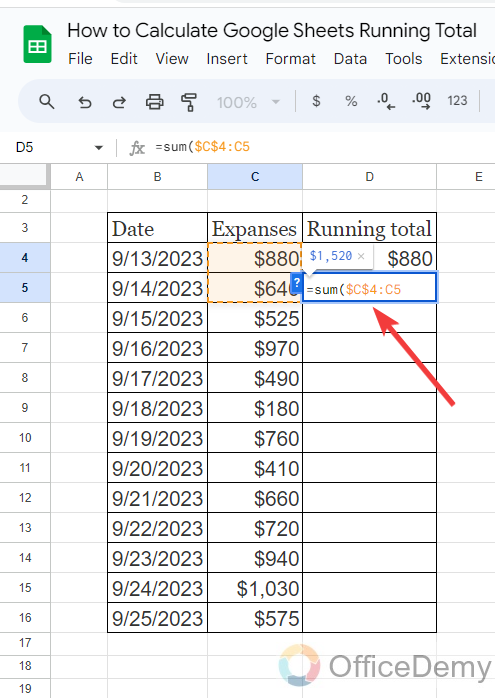
Step 5

Now, you can press the Enter key to get the result as you can see in the following picture, now just drag this formula over the other cells to calculate other values of the running total.

Step 6

As the result is in front of you as you can see in the following screenshot, we have all the values for running total according to expenses with an array.

3. Dynamic Running Total

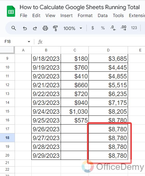
Let’s suppose, you are calculating a running total daily expense, and one day you don’t spend a single penny, and your expenses cell is empty for that day how will you get the running total for the next day, it will turn into an empty cell or will give you the same value. In such a situation, we apply the following method of calculating the running total in Google Sheets. Although the above two methods are fine for calculating the running total in every aspect if you don’t want to display the same values in the cell or to show anything else when the expense is empty then this method is helpful.

Step 1

If you see in the following example when we drag the formula over the extra cells, it gives the same value in the other cell instead of empty.

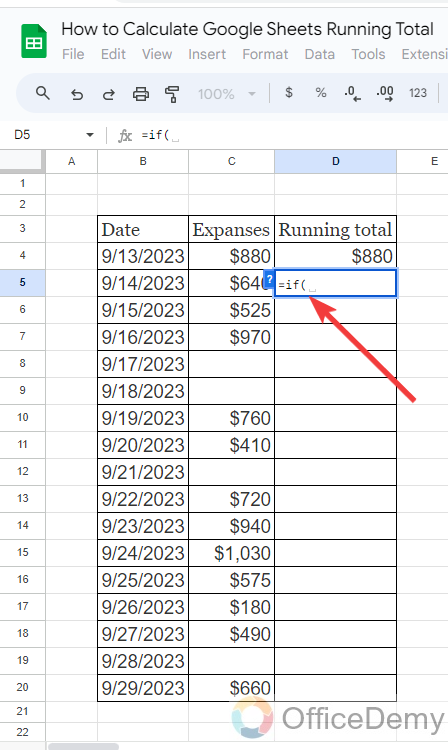
Step 2

To apply the dynamic running total in Google Sheets, we will use the “IF” formula as directed below. In this method as well, we will write the first value as it is in the first cell then will apply the formula in the second cell.

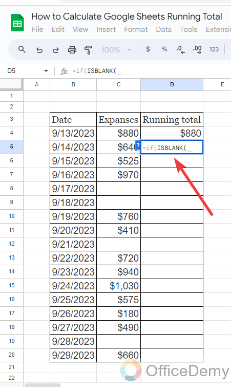
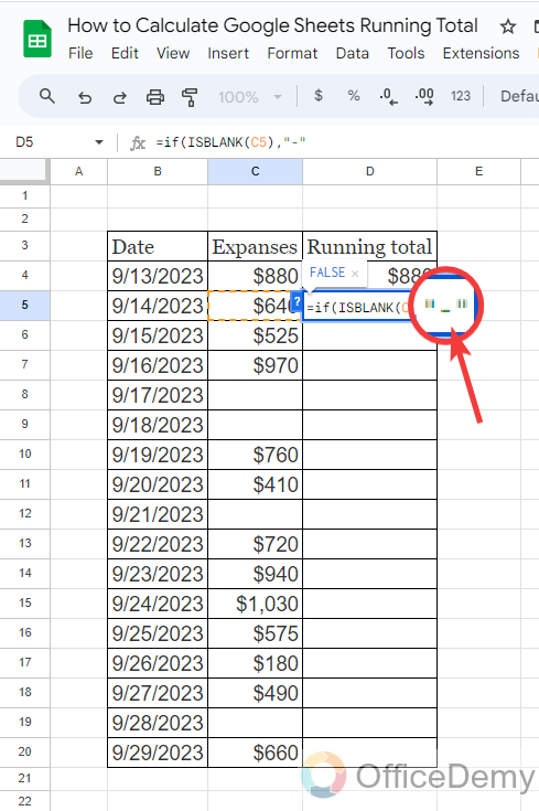
Step 3

After starting the “IF” function, we will add another function of “ISBLANK” in the syntax as written in the following picture.

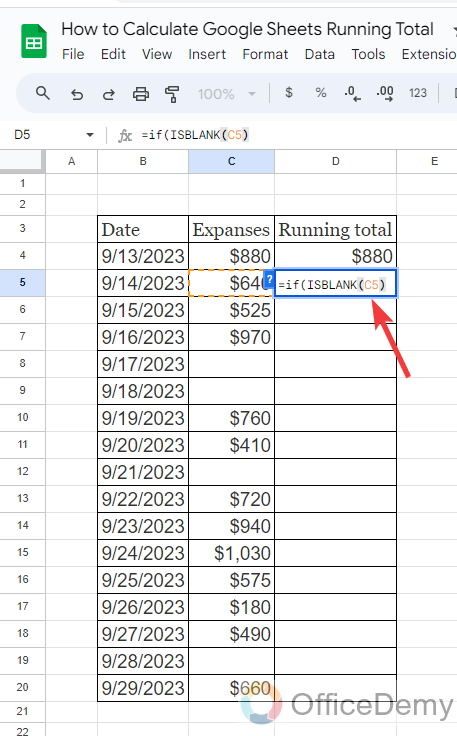
Step 4

First, we will complete the second “ISBLANK” function by giving the cell reference of the data value that is expensed in the following example.

Step 5

After giving the data value, according to the “ISBLANK” function syntax, we will give the criteria as here I am writing “–“. It means, that when there will be the cell empty it will automatically insert the dash mark into the cell as per the given.

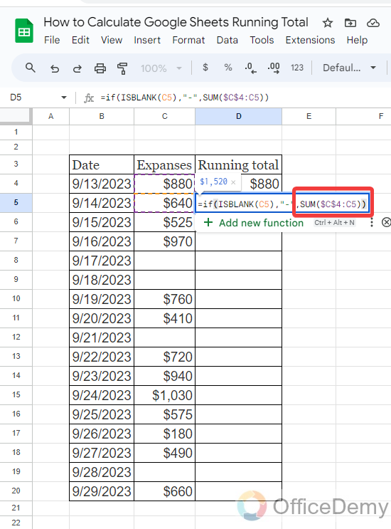
Step 6

Now, we will complete the first function by giving the second condition in the syntax which is the simple sum formula of calculating the running total as highlighted.

=IF(ISBLANK(C5), ” – “,SUM($C$4:C5))

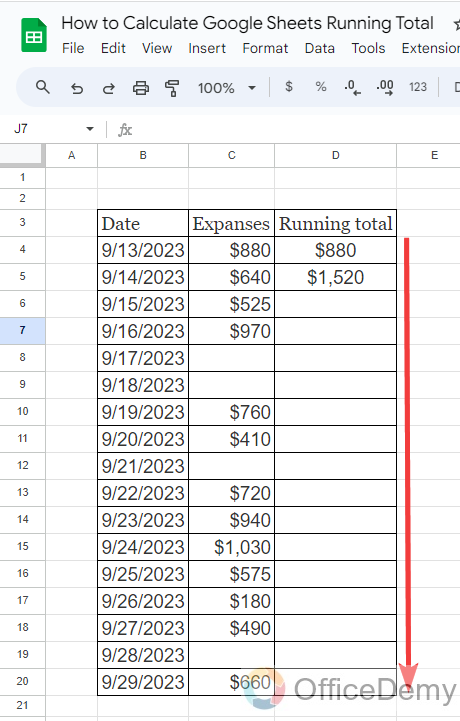
Step 7

Once you have completed the syntax, then close the bracket and hit the Enter key to get the result. Once you have gotten the first result, drag this formula over the other cells to get the other values of the running total.

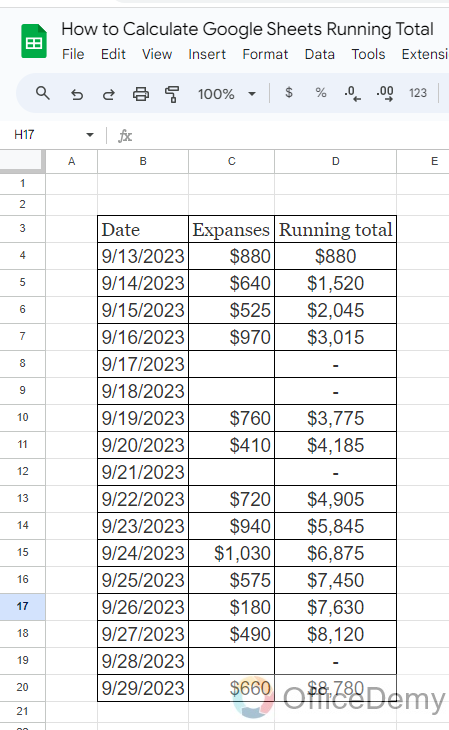
Step 8

You should get the result below, as we can see below where the cells are empty, we are getting a dash mark

Frequently Asked Questions

Can Rounding Numbers Affect the Accuracy of Google Sheets Running Total Calculation?

To avoid any discrepancies, it is crucial to stop rounding in google sheets when calculating running totals. Rounding numbers may lead to small errors accumulating over time, impacting the accuracy of the overall calculation. Beware of the potential pitfalls and ensure precise calculations by disabling rounding in Google Sheets.

Conclusion

In this tutorial on how to calculate Google Sheets running total, we have covered three different methods of calculating the running total, you don’t need to get confused and can use any of them according to your preference.