To Alternate Row Color in Google Sheets
Alternating Colors Option:
- Select Data.
- Go to the “FORMAT” > “Alternating Colors“.
- Select a color and check the “Header” and “Footer” options if needed.
- Click “Done” to color alternate rows quickly.
Conditional Formatting for Alternating Rows:
- Select Data > Go to the “FORMAT” > “Conditional Formatting“.
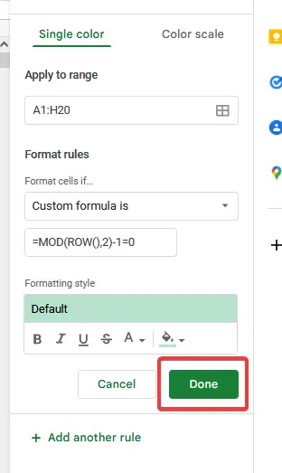
- Select “Custom formula is” from the format rules.
- For coloring, use the formula =MOD(ROW(),2)-1=0 > Apply and Customize.
- Click “Done” to apply the formatting.
In this article, we are going to study some formatting features of Google sheets that show how to color alternate row in Google sheets. Now in Google Sheets it is quite easy to color alternate rows because there is a separate option in the Google sheets tab menu for alternating colors which is not found in other software.
As Google Sheets is providing their users formatting features to make their documents beautiful and presentable in which color alternate rows is one of them in which you may highlight the rows with different colors to make your document more attractive, it can be used for separation of rows as well or other purposes as you desire.
Why we need Alternate Row Colors in Google Sheets?
Google sheets is an online web-based spreadsheet program providing the features of editing and calculating or analyzing some kind of financial data etc. We may not forbid that there is no need of formatting our documents. Besides, it is essential sometimes to make documents more presentable, so there you might need this feature to color alternate rows in Google sheets.
By coloring alternate rows you may highlight your data or table and can make it easily readable and to find something. It also helps to show separately individual rows in your data. There are so many scenarios where you may need to color alternate rows as you required.
How to Alternate Row Color in Google Sheets
Alternate Row Color in Google Sheets – using Alternating Colors option
As I told you in Google sheets, it is quite easy to color alternate rows because Google sheet provides a separate option in its tab menu to color alternate rows within a few clicks but there are some more customization options in the “Alternating Color” dialogue box which we will discuss in detail. And here I will also teach you a conditional formatting method to color alternate rows or any row you want to color or highlight. So let’s start without wasting our time
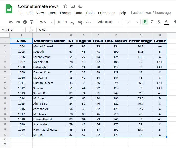
Step 1
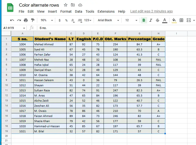
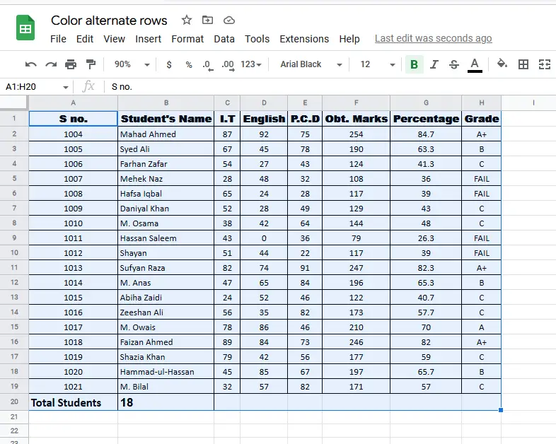
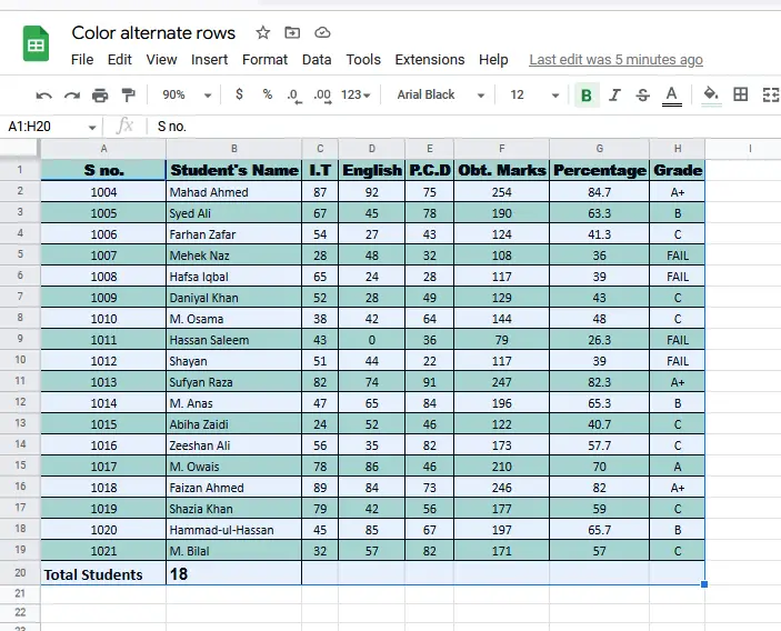
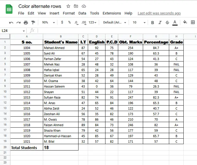
First we will take some sample of data and select it all
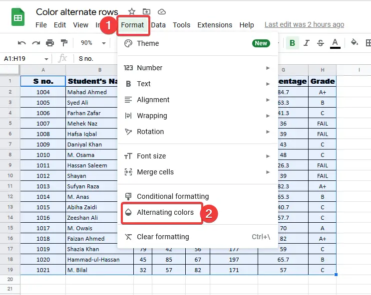
Step 2
Go to the tab menu “FORMAT” and find “Alternating Colors” and click it to open
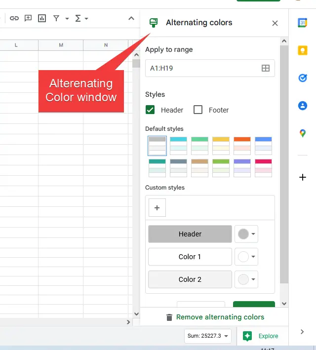
Step 3
A dialogue box or a pop-up window will appear on the right side of your Google sheets where you will find some customization options
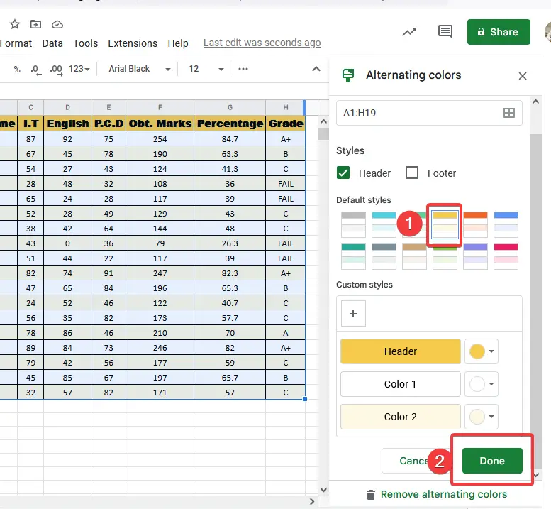
Step 4
Now in just a few clicks you may color alternate rows, First select the color you want to apply and then just click “Done” as you may see below
Step 5
As you may see that you are done now, your rows have been colored alternatingly.
Alternate Row Colors in Google Sheets – Alternating Colors Additional Options
As you have seen how quick it is done in just a few steps although there are so many customizations in Alternating colors you should know them so let’s do a brief discussion one by one,
Cell range
First, we find cell range in the Alternating Colors dialogue box where you may insert cell range or an area where you want to apply the alternate colors rows
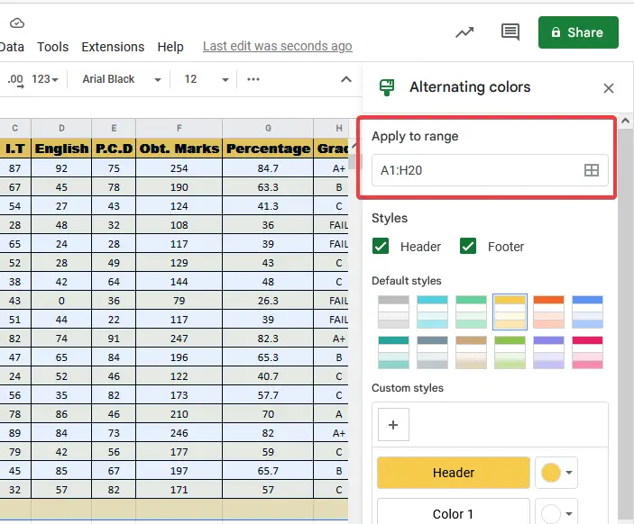
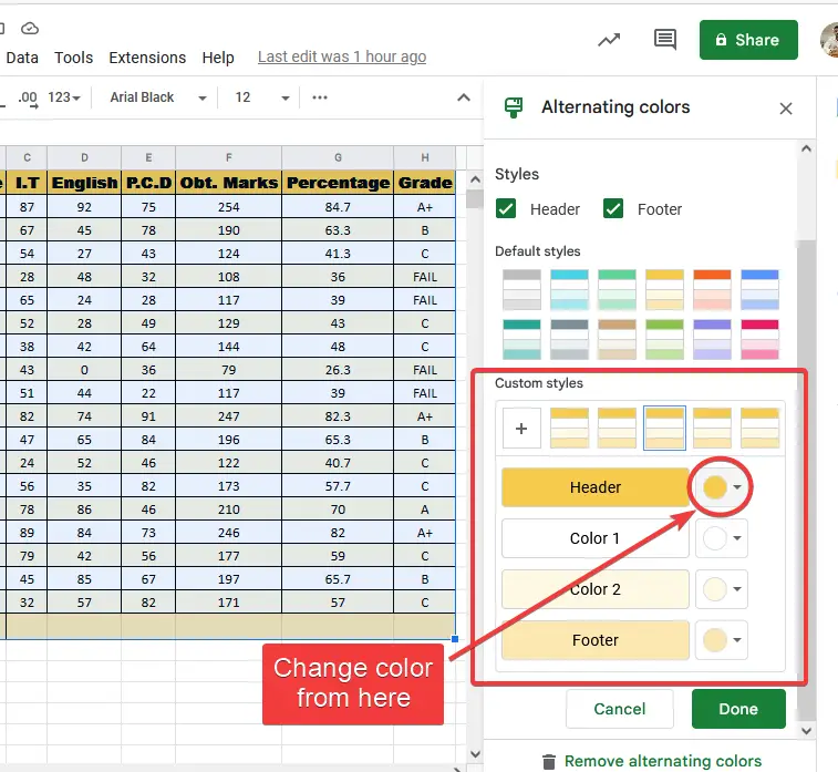
Styles
This is a very good and useful option available in Alternating Colors consisting of two buttons with a checkbox “Header” and “Footer”. As we usually have in our data or a table, headings at the top and conclusion in the bottom like total etc. in bill or etc. Sometimes we need to highlight them, or sometimes we do not need to color or highlight them, it also depends on our preferences that How we want to format our document
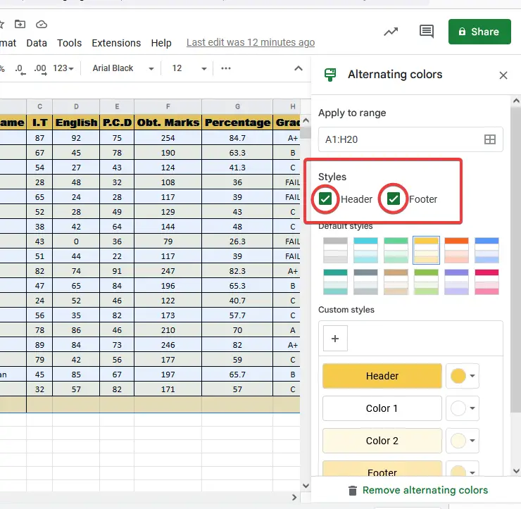
So you don’t need to worry at all just you may do it by one click on it by checking or unchecking the box, your headings will highlight if you checked the header button or it will not if unchecked the same button similarly for the footer.
Default Styles
In the next section, we find some styles by default formatted of different colors tones, from which you may choose any of them you like
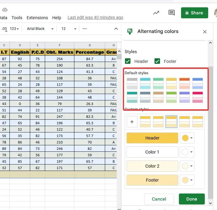
Customs Styles
If you don’t like any of the default styles so in just the next section you may customize it with your own desire, You may change the color of every row what you want like
Here we have completely learned the “Alternating colors” in Google sheets we learned how to color alternate rows and also we learned the all customization of alternating colors. With all above lesson there will not be any problem to color alternate rows, It will help you in all scenarios.
Alternate Row Color in Google Sheets – using Conditional Formatting
Yet! I have covered my topic in the above lesson about how to color alternate rows in Google sheets but there is one more method by which you may color not only alternate rows but also any row that you want to color. Google sheet inserts the option of alternate colors later it used to be done by conditional formatting before. Our topic is related to color alternate rows but by this method we may also color every third or fourth row in our data sheet. This method is a little complex because of using syntax for rows but we will study it with complete guidance and examples so you may learn and can easily apply it to your documents.
Syntax
=MOD(ROW(),2)-1=0
This formula is used to get the row numbers.MOD formula is used to divide the specified divisor which is number 2 in the above syntax and the remainder will be 1 because we are writing the formula to color alternate row or every other row
Similarly, if we want to color the row in such a pattern that every third row will be colored then the syntax will be
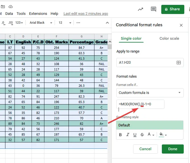
=MOD(ROW(),3)-1=0
And similarly further so on you may customize as you want, let’s start with step by step procedure,
Step 1
As usual, first, take a sample of data and select all of the data you have
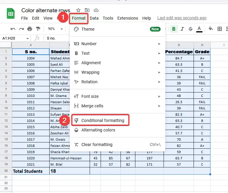
Step 2
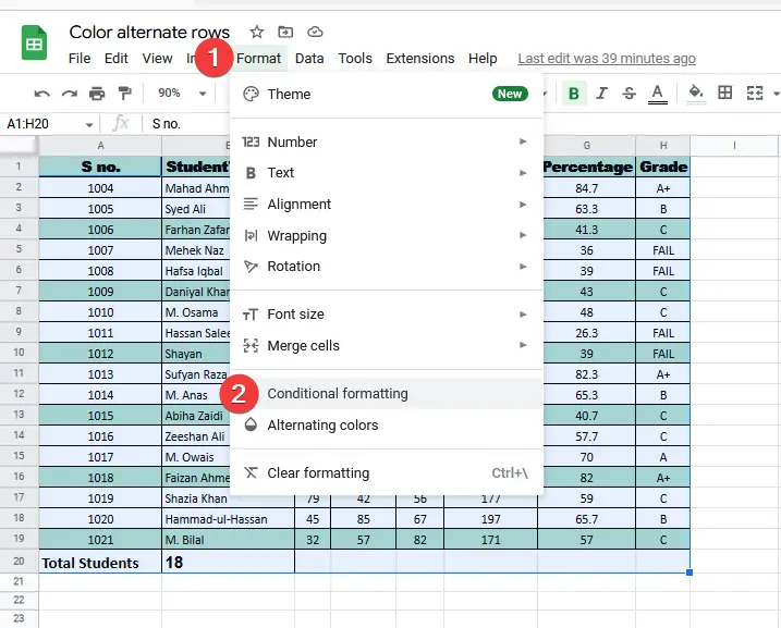
Similarly go into the “FORMAT” tab from the menu and find open the “Conditional Formatting” just above the alternate colors
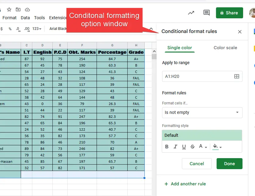
Step 3
A pop-up window or dialogue box for Conditional formatting will appear on the right side of the Google sheets
Step 4
Now it is time to apply conditional formatting by selecting first “format rules”.
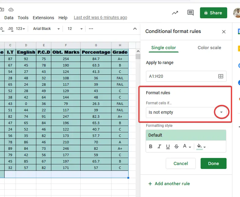
Step 5
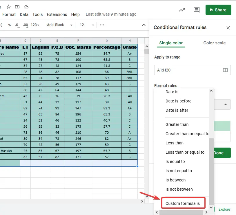
Select the format rule to “Custom formula rule” because we will insert the formula manually for rows that we want to color
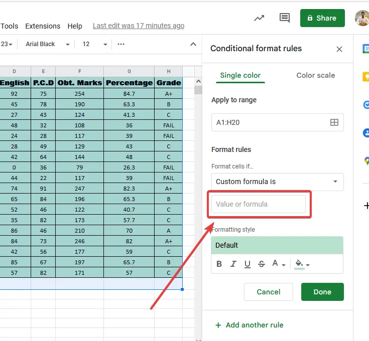
Step 6
There you will found another box where you will write you customs formula
Step 7
Now you will find little difficulty while inserting formula but once you understand the logic it will be pretty easy, If you want to color alternate rows then the syntax will be
=MOD(ROW(),2)-1=0
Write the formula in the formula bar
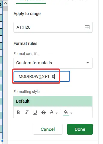
Step 8
Now simply press the “Done” button
Step 9
Here, you may see the result you have colored alternate rows
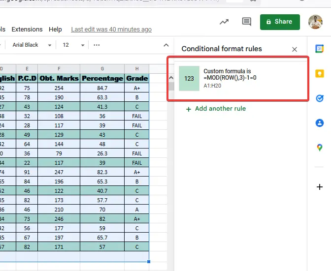
Alternate Row Color in Google Sheets – Color Every Third or Fourth row
If you want to color every two rows of three then repeat the same above procedure just change the syntax like,
=MOD(ROW(),3)-1=0
You may see in the above picture that every third is highlighted or colored. In such a manner you may further customize or color your rows and make your document beautiful and presentable.
Tips:
You may also do some more formatting by this conditional formatting method,
- You may also use some default formulas and conditional formatting rules
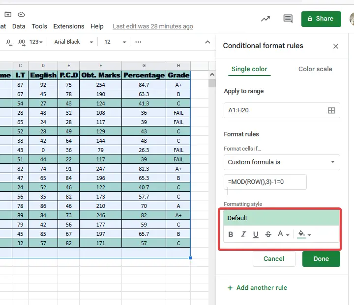
- Firstly you may select any of the colors that you want to color your rows.
- You may also Bold, Italic, and underline your text.
- You may also change font styles by this formatting.
- There is a strike-through button that is also available to strike through the text.
Here you may find all these options
Alternate Row Color in Google Sheets – How to Remove Conditional formatting
Once you have applied conditional formatting and then if you want to remove the customization to retrieve your documents in their original condition so you may easily delete them within a few steps let’s see
Step 1
Go to the “FORMAT” tab in the menu and go to the “Conditional Formatting” from the drop-down menu
Step 2
A pop-up window will open on the right side of your Google Sheet where you will find a pane saved of your editing as you may see below.
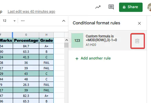
Step 3
To delete this formatting simply move the cursor to the pane of formatting, You will see a trash button press it to delete the formatting as you may see in the picture
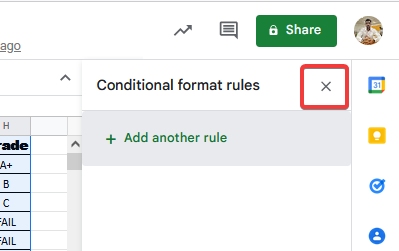
Step 4
Now, close the formatting window
Step 5
You have successfully deleted the all formatting rules now here is your document in its original condition
Important Notes
- If you have formatted your cells or colored your cells or rows already and then you apply the “Alternating colors” or “Conditional Formatting” so it will be overwritten on it, your previous editing or formatting will be hidden automatically.
- Once you apply “Alternating colors” or “Conditional formatting” on a table or rows and then you expand it to more rows so it will automatically adjust the color pattern and similarly if you delete your data as well
Conclusion
As we find how to color alternate rows in Google sheet is very useful to make our documents beautiful and presentable. This is why I wrote this article in which I covered all scenarios to color alternate rows and as well every third or fourth row by the Alternating colors method and Conditional formatting method. I hope you understand better with my given examples and shall not have any problem while applying the above conditions or formatting to your data.
Thankfully don’t forget to give thumbs up, like, and subscribe.


