
To Generate a Random Number in Google Sheets
- Start the RAND function.
- Keep the brackets empty.
- Press the Enter key.
OR
- Start the RANDBETWEEN function.
- Write the lower limit and upper limit.
- Press the Enter key.
OR
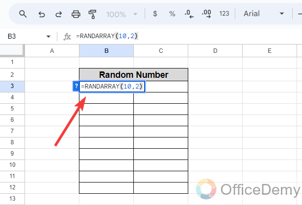
- Start the RANDARRAY function.
- Write the nth number of rows and columns.
- Press the Enter key.
If you need to generate a random number in Google Sheets, fortunately, Google Sheets provides three functions for randomly generating numbers, the first is RAND, RANDBETWEEN, and then RANDARRAY. Today in the following guide on how to generate a random number in Google Sheets, we will discuss all these three functions in detail.
So, let’s get started without wasting our time.
When we need to Generate a Random Number?
There may be so many reasons to generate a random number in Google Sheets, that you may need it for testing codes, playing dice, and sample datasets. These random numbers can be useful for some statistical methods in Google Sheets.
So, if you also need to generate random numbers in Google Sheets read the following guide on how to generate a random number in Google Sheets.
How to Generate a Random Number in Google Sheets
Google Sheets has three different defined functions to generate a random number. Let’s see how to use them in the following guide.
- By using the RAND function
- By using the RANDBETWEEN function
- By using the RANDARRAY function
1. Generate a Random Number with the RAND function
The most common way of generating a random number in Google Sheets is by using a Rand function of Google Sheets. The RAND is a number Libra function that can give you a positive random number between 0 and 1. Below are the steps to use the RAND function to generate a random number in Google Sheets.
Step 1
Let’s suppose, we have to generate a random number in the following cell as directed below. To generate a random number in the next cell box, place your cursor in the next cell.
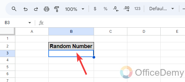
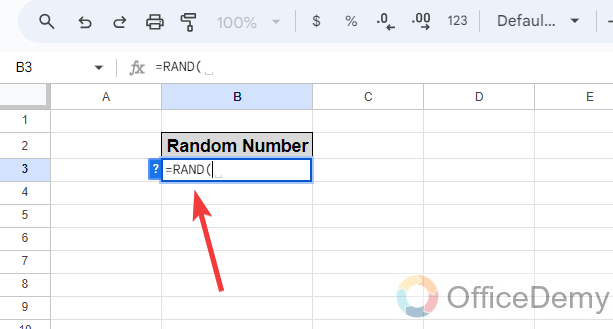
Step 2
After placing the cursor in the cell, we will start the RAND function by just writing RAND with an equal sign as I have written in the following picture. After starting the RAND function, leave the brackets empty.
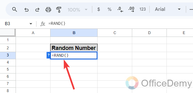
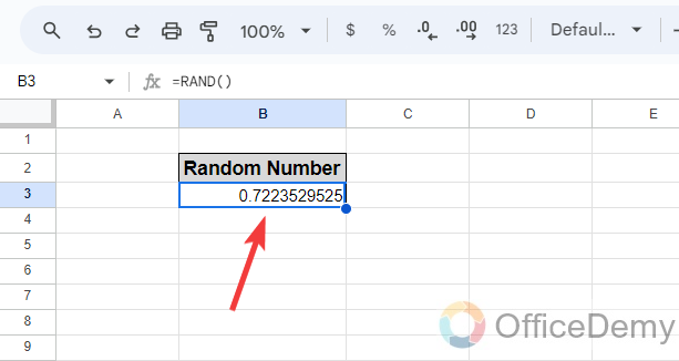
Step 3
Once you have written the formula of the RAND function, as you press the Enter key, you will get the random number instantly as we have gotten in the following picture.
2. Generate a Random Number with a RANDBETWEEN Function
The above RAND function of Google Sheets is effective in generating a random number in Google Sheets but it gives you a random number only between 0 and 1. If you want to get a random number greater than 1 then you will have to use the RANDBETWEEN function of Google Sheets, it cannot only give you a random number greater than 1 but also enable you to specify the lower limit and upper limit to get the random number in between. Here we will learn how to generate a random number by using the RANDBETWEEN function in Google Sheets.
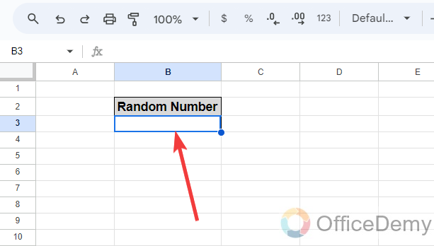
Step 1
Firstly, place your cursor where you want to generate a random number between the two values in the cell as I have selected in the following picture.
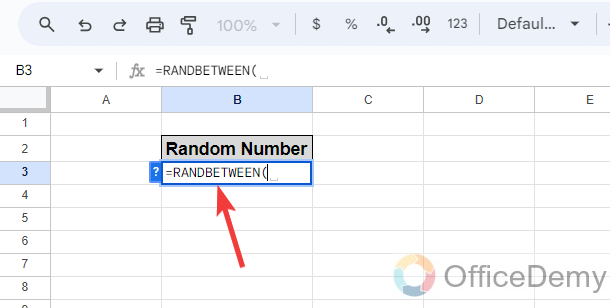
Step 2
Once you have placed your cursor in the cell then run the RANDBETWEEN function in the cell as I have written in the following picture.
Step 3
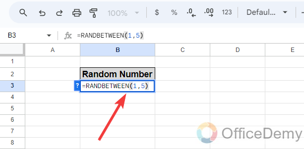
As we are generating the random number between two values here, we will specify those two values in the RANDBETWEEN function in the following pattern first you will write the small value and then the large value as written below.
Step 4
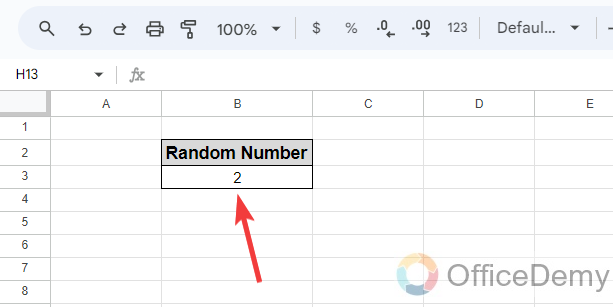
In this way, you will get the random number between two values as we have put 1 to 5, so here we have got “2” as displayed in the following picture.
3. Generate a Random Number with the RANDARRAY Function
The RANDARRAY function is just an array form of the RAND function of Google Sheets, it also gives you a random number between 0 and 1 but you can get multiple random numbers in an array with the help of using the RANDARRAY function of Google Sheets. There is a complete guide regarding the RANDARRAY function in the following steps.
Step 1
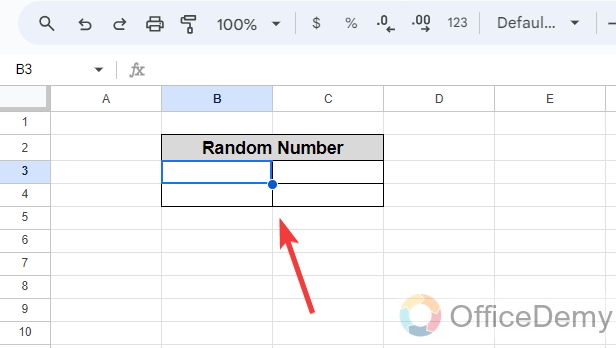
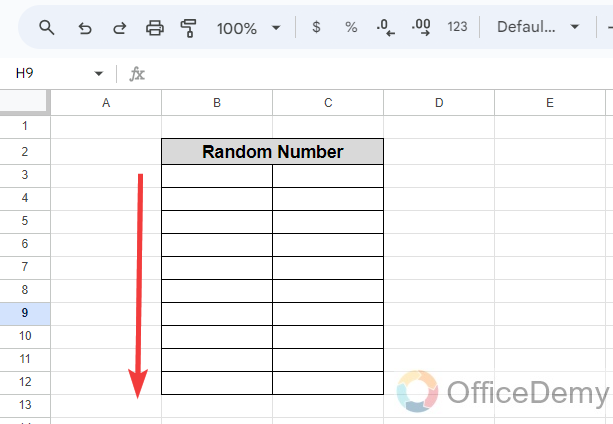
Let’s suppose, there are two rows and two empty columns where we want to generate the random numbers so we will use the RANDARRAY function of Google Sheets.
Step 2
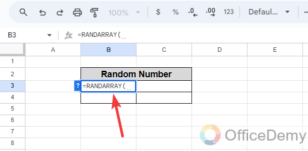
Similarly, first, we will run the RANDARRAY function in the first cell by just writing RANDARRAY with an equal sign as I have written in the following picture.
Step 3
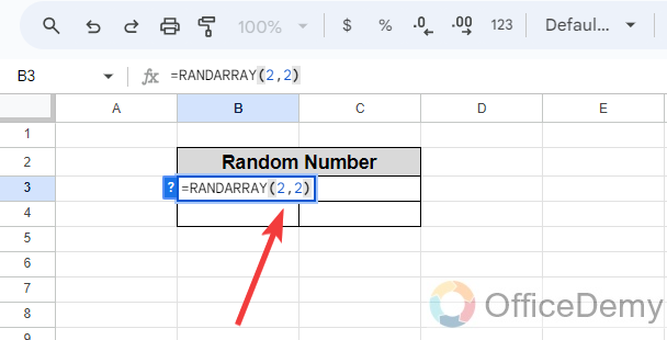
In the syntax of the RANDARRAY function, there are only two arguments which are the nth number of rows and columns. Here we want to generate random numbers in two rows and columns so we will write “(2,2)” as can be seen in the following picture.
Step 4
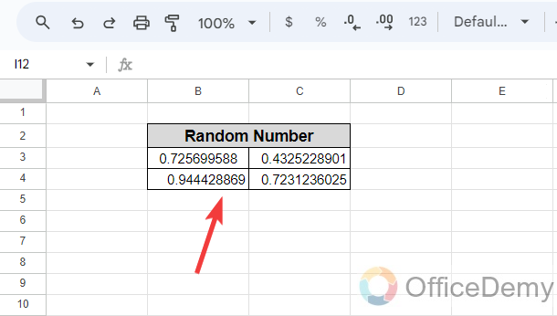
When you press the Enter key, it will give you the result as follows as can be seen below here we have gotten random numbers in two rows and two columns.
Step 5
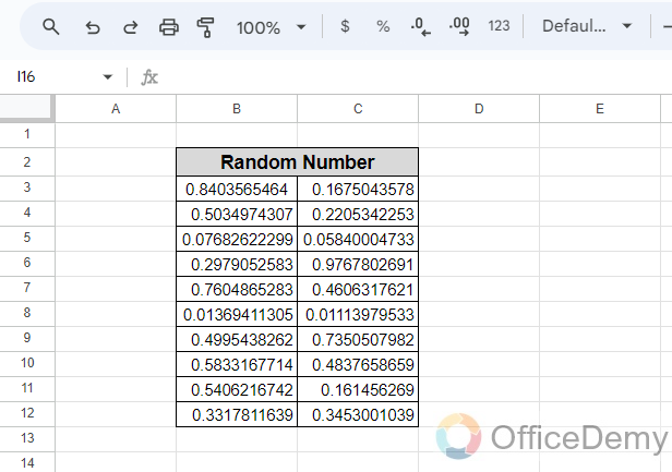
In the same way, if you want to generate random numbers in the ten rows and two columns then you can also even generate random numbers between ten rows and two columns.
Step 6
To generate random numbers between ten rows and two columns, we must write the string in the syntax in the following pattern as written in the following picture.
Step 7
Now, you will get random numbers between 10 rows and 2 columns when you press the Enter key as you can see the result below.
Frequently Asked Questions
How to combine RAND and RANDBETWEEN to generate random numbers in Google Sheets?
As we have discussed above as well, the RAND function generates only a random number between the values 0 and 1. But we can also generate random numbers between two values with the help of a combination of RAND and RANDBETWEEN functions in Google Sheets. Let me show you how to combine the RAND and RANDBETWEEN functions of Google Sheets.
Step 1
Place your cursor where you want to get the random number by using the combination of RAND and RANDBETWEEN functions in Google Sheets. First, we will start the RAND function in the cell as written below.
Step 2
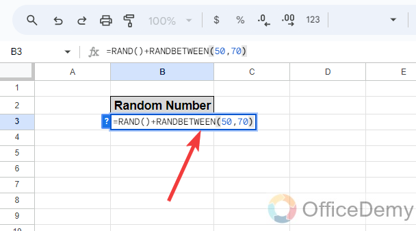
We will leave the brackets of the RAND function empty and then will write an additional sign in the syntax as I have written in the following picture.
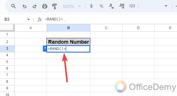
Step 3
After the addition sign, start the RANDBETWEEN function by simply writing RANDBETWEEN. After starting the RANDBETWEEN function, write the values in which you want to generate the random numbers.
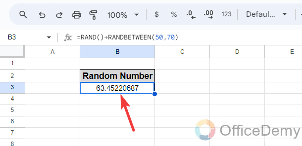
Step 4
You are almost done with writing the syntax, then when you press the Enter key, you will get your random number as highlighted in the following picture.
How to find the random number between the values by using the RAND function?
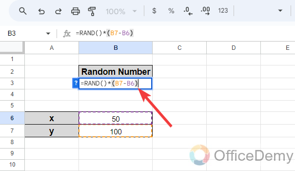
Let’s suppose, you already have two different values X and Y, and you want to generate a random number between these two values X and Y then you can use the following formula to find the random number between X and Y as follows.
Formula: =RAND()*(Y-X)+X
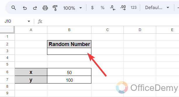
Step 1
To find the random number between the values by using the RAND function in Google Sheets, you will need to write both values in a separate cell to give reference then apply the syntax in the following directed cell.
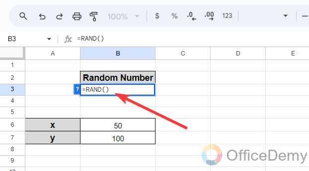
Step 2
Simply, first, write the RAND in the same previous way, as noted in the following picture.
Step 3
According to the syntax, here we will add a multiplication sign and then add the expression “Y-X” As you can see in the following picture, I have given the cell reference of x and y.
Step 4
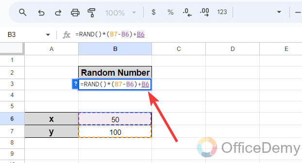
In the last, you will have to add x in the resultant value so here we will add an addition sign and then will give the cell reference of x as written below.
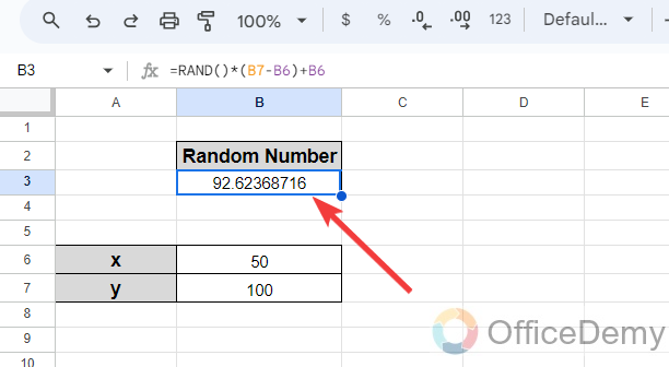
Step 5
Now just have one click to go, as we press the Enter key, we will get the random number between the specified values as can be seen below.
Conclusion
In this tutorial, we have discussed different functions that are used to generate random numbers in Google Sheets. We hope you find this guide on how to generate a random number in Google Sheets helpful to you.


