How to Make Negative Numbers Red in Google Sheets [2 Methods]

In this article we will learn about how to make negative number red in color in Google Sheets. Google sheets are mainly used for calculating, analyzing, and producing charts and data consists of the majority of numbers and values. It can be a basic payroll, calculating revenues, calculating taxes, billing, reporting, etc. We usually have large numbers of data in the form of numbers including both kinds of values negative and positive.

Sometimes it does need to highlight negative numbers to indicate them separately so we may find and monitor them easily. As generally negative numbers are always indicated by red color, in this article, we will learn how to show negative numbers in Google sheets. So that you may traditionally customize your spreadsheet data for an attractive and professional visual.

Why making Negative Numbers Red is important in Google Sheets?

As I discussed in Google sheets, we usually work on most numeric data which includes every kind of number. There are positive values and negative numbers as well. In this boosted era of technology and functionality If we find negative numbers one by one in a huge bulk of data, it costs a lot of time which is not suitable. Therefore, there are very helpful features available in Google sheets by which we may efficiently find negative numbers by formatting them in red color. This is why we need to learn how to show negative numbers in red in google sheets.

How to Make Negative Numbers Red in Google Sheets

Google sheets provide their user with countless features of formatting your data in your way. And also, there are many and simplest methods to apply any kind of formatting in Google sheets, similarly, there are two methods to show negative numbers in red color in google sheets,

1. Show Negative numbers in red by conditional formatting
2. Show Negative numbers in red by customs formatting

Both methods have similar and dynamic results and both are easy to apply, you desire that you prioritize which one of them. We will deeply discuss them one by one with the simplest example and complete guidance while you learn it quickly.

Make Negative Numbers Red in Google Sheets – using Conditional Formatting

Conditional formatting in Google sheets by default includes many rules to format your data in the manner that you want. Just we have to understand the logic of formatting that we require and then apply the condition accordingly. Don’t worry we will clear you all the logic of conditional formatting in a step-by-step procedure.

Step 1

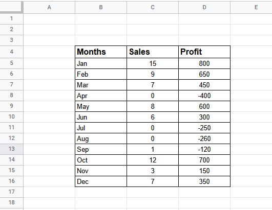
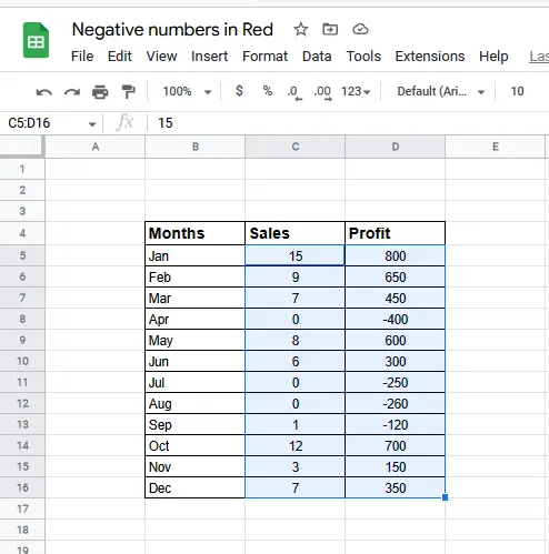
First, let’s have a sample of data where you want to highlight the negative numbers but make sure your data must have some negative values.

Step 2

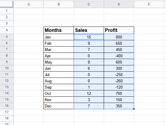
Now select the data or range where you want to apply conditional formatting to show numbers in red

Step 3

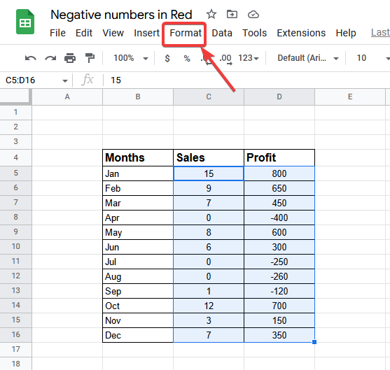
Now simply go to the “FORMAT” tab in the tab menu.

Step 4

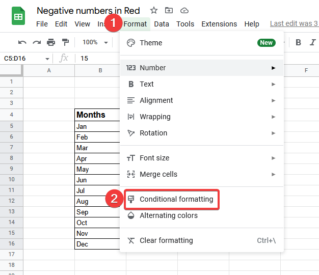
As we are applying conditional formatting, find the conditional formatting button in the drop-down menu and open it by clicking on it.

Step 5

Once you click on the conditional formatting option a separate window will open on the right side of the google sheet for conditional formatting rules.

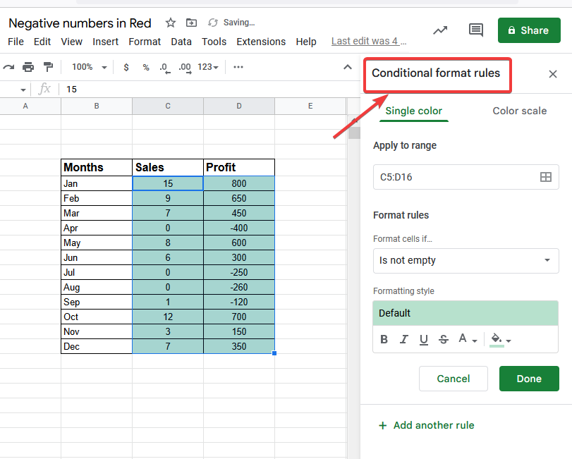
Step 6

Now find format rules in this window to choose the condition you want to apply.

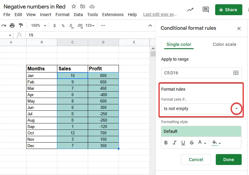
Step 7

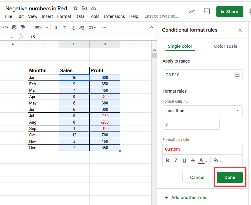
Now there is quite easy logic to find your condition as we know that we are looking to show negative numbers in red so how may we input the condition of negative numbers in format rules?

As we know that all negative numbers are less than 0, so we may apply the condition of less than and can use the value 0 to find out all negative numbers. Let’s do that practically,

First, find the condition of less by scrolling down in the format rules

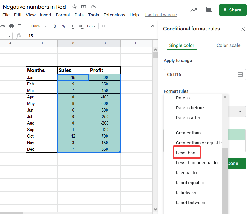
Step 8

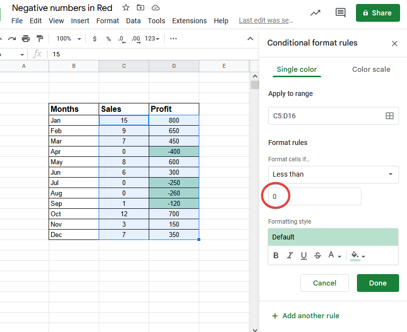
We are looking for all negative numbers, so here we will put the value ‘0’,

Note: We used the value ‘0’ as we need all negative numbers. You may also use any value here according to your condition. If you need all values that are less than 100 you may put ‘100’ instead of ‘0’.

Step 9

Your condition has been applied, google Sheets has found all negative numbers in your selected data. Now we need to color all negative numbers in red. So to color, the number, find the text color option in the next section of format rules and open it.

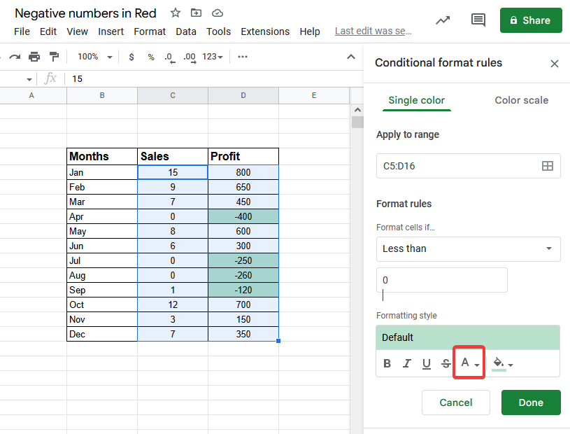
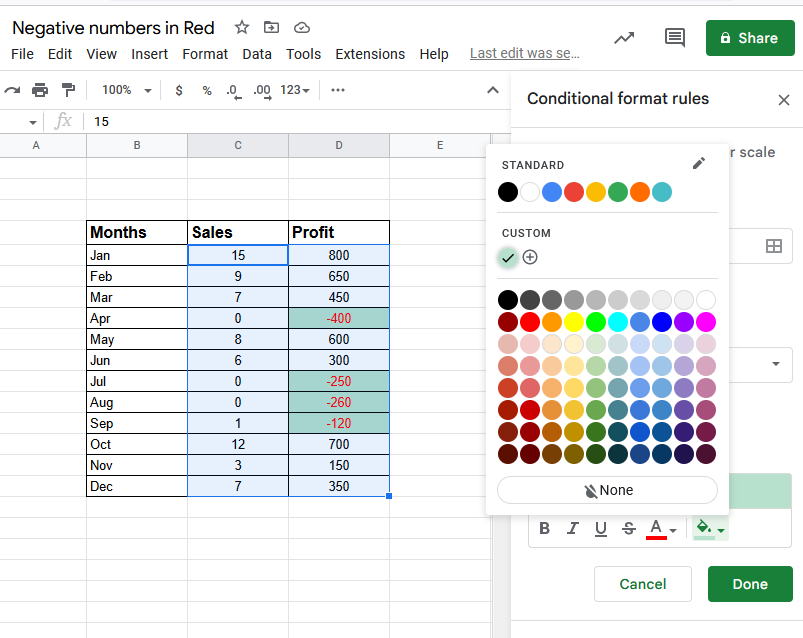
Step 10

You will have different colors here, but we need red color so we will select a red color.

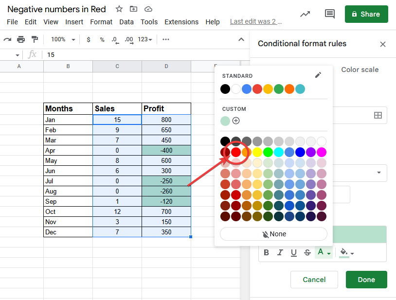
Step 11

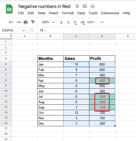
Now you may see here that all negative numbers are being shown in red solar as we require.

Here by default, you will find all formatted cells filled by some color If you want to remove it you may simply fill it in white color like

Step 12

Where you found the text color option, In just right you will find the color fill option.

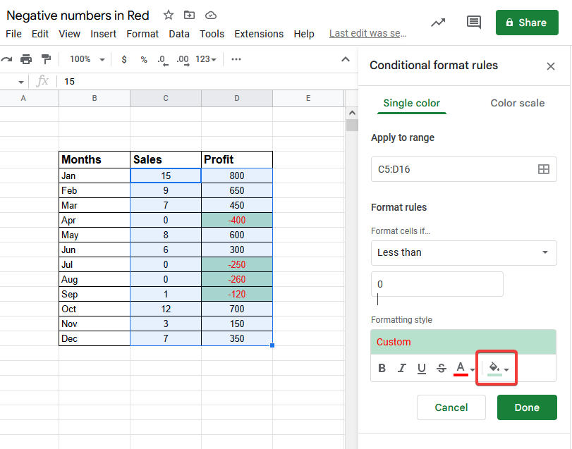
Step 13

Simply open it and select the white color if you want to remove the cell fill color or select any color that you want to fill with.

Step 14

After applying all conditions just press the “Done” button to end the procedure.

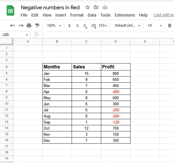
Step 15

You have your desired data as negative numbers are in red.

Make Negative Numbers Red in Google Sheets – using Custom Formatting

This method of how show negative numbers in res in google sheets is also based on some logic by default installed in google sheets. In Google sheets especially in customs formatting, there is a sequence pattern of text and numbers like, (Positive number, Negative number, zero values, text), and every argument is separated by a comma (,). It will help while applying the condition in custom formatting. Let’s make a better understanding with the help of some examples.

Step 1

As usual, first, select the data where you want to apply the formatting rules.

Step 2

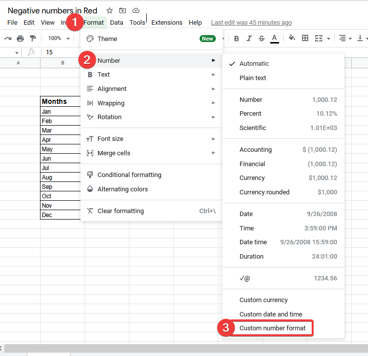
Now again go to the “Format” tab and find “Number”.

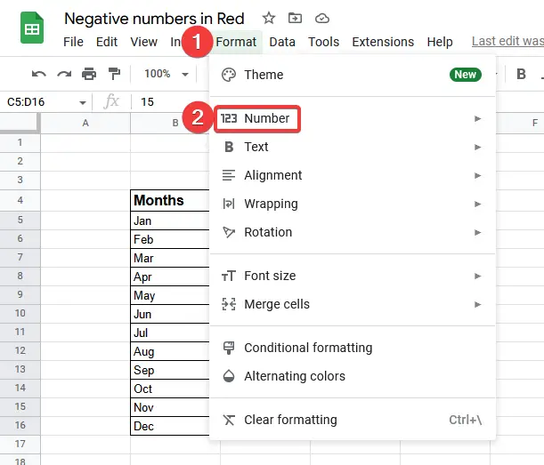
Step 3

As you click the number the 2nd drop-down menu will open where you will find “ Custom number format” at last.

Step 4

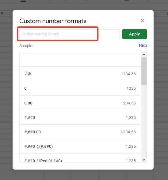
A pop-up window will appear where you will find a dialogue box in front of you where you will write the condition that you want.

Step 5

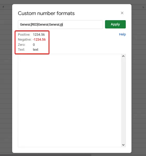
Here you have to write a custom formatting rule, as we discussed there is such a pattern in which there is a sequence which is (Positive number, Negative number, zero values, text, now here we need to color just negative number so we will write the rule in such a manner that (General;[RED]General; General;@),  As the negative number is 2nd argument so we wrote: “RED” in a 2nd argument which will format negative numbers in red color, where “General” is representing general (by default) formatting which will remain same while “@’ is representing text.

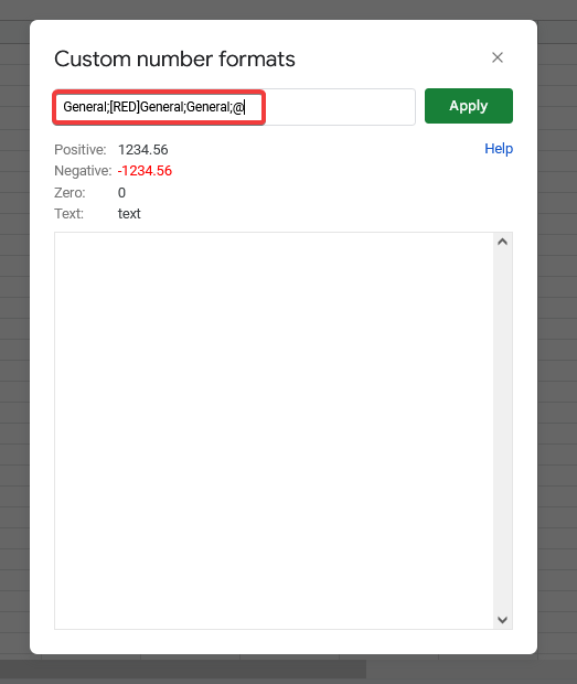
Tip: Must use the square brackets “[]” while writing the color name.

Step 6

You may also verify the pattern or formatting you applied below as shown in the picture the negative numbers are in red color which means your syntax is correct.

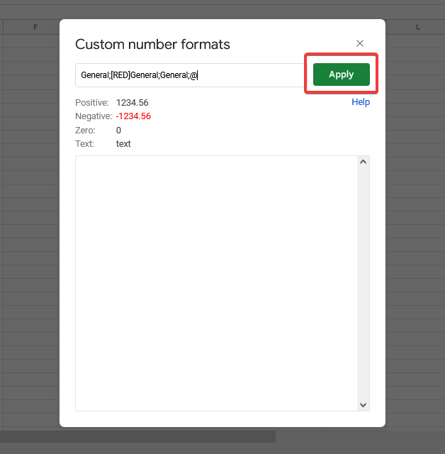
Step 7

Once you verify the condition then just simply press the “Apply” button to finalize the process.

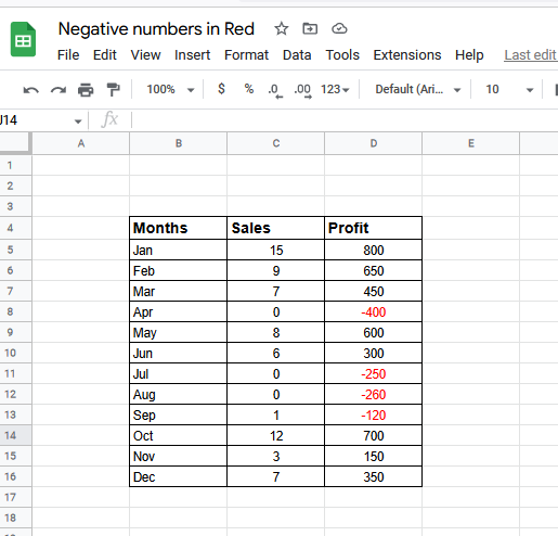
Step 8

Here is the result that you require all negative numbers are shown in red color.

As we have finished both our methods, I prefer the conditional formatting method instead of custom formatting because it is easy to use and more reliable.

Important Notes

Frequently Asked Questions

Why do we need to show negative numbers in red?

When working with a large data set where negative and positive values are together in a column or list, we need to ensure the negative data is separated from the positive one so we cannot have any calculation errors. We have seen two easy methods to do it and it helped us highlight the negative numbers with any color, essentially the red to that the values are negative

Can we show positive numbers in green in google sheets?

Yes absolutely, you have these two methods not limited to showing only negative numbers to red, you can show positively in green, bigger values in yellow, and any combination of condition and value you can make using the above methods.

Conclusion

Wrapping up how to make negative numbers red in google sheets. We have learned how to use the above two easy methods to show negative numbers in google sheets. I hope you find the above explanation helpful and useful. for more similar content and helpful tutorials, consider subscribing Office Demy blog. I will see you soon with another helpful article. Thank you & Keep learning with Office demy.