How to Use Wildcards in Google Sheets [Full Tutorial]

Today, we will learn how to use Wildcards in Google Sheets. Wildcards are like a symbol in Google Sheets that are used to represent a character or number of characters enabling you to get the relevant results. In this article on how to use wildcards in Google Sheets, we will learn how we can sort our queries with the help using these wildcards. So, let’s get started without wasting our time.

Benefits of Using Wildcards in Google Sheets

The most benefit of using the wildcard in Google Sheets is while searching or sorting a query from the data. When you are making an operation in Google Sheets and you are not aware of the exact value or character, it helps you to place a string in substitute of a certain character or set of characters. You can find your query even with incomplete information by using Wildcard in Google Sheets.

Let’s see how to use wildcards in Google Sheets in the following tutorial.

How to Use Wildcards in Google Sheets

There are only three wildcards used in Google Sheets. In the following tutorial on how to use wildcards in Google Sheets, we will learn all of them one by one and step-by-step with the help of examples.

• Asterisk (*)
• Question Mark (?)
• Tilde (~)

How to Use Wildcards in Google Sheets – Using Asterisk (*)

In Google Sheets, as a wildcard, an asterisk can be used to represent any symbol or number of characters. If you don’t know the exact number of characters, letters, or symbols, you can stand an asterisk sign. Let me show you practically with the help of the following couple of examples.

Example # 1

Step 1

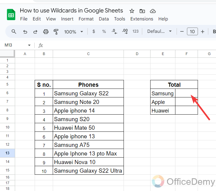
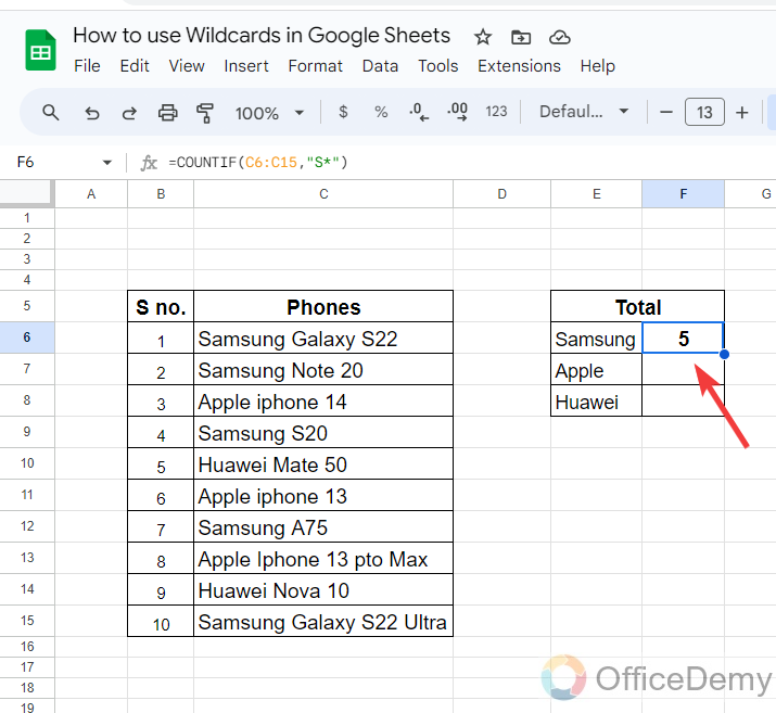
In the following picture, see, there is a data table of different brands of mobile phones, while on the other side, there is another small table where we have to count all mobiles of individual brands. Let’s see, how to use wildcards in Google Sheets in such a situation.

Step 2

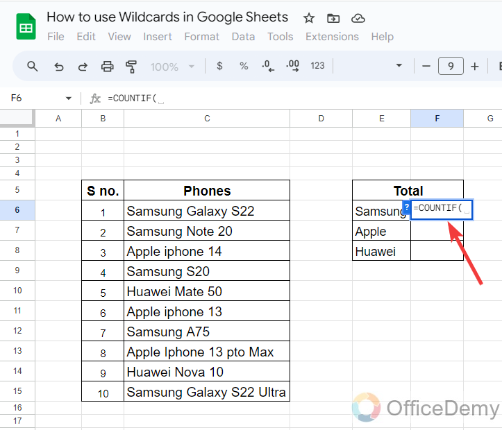
Here, we will use the COUNTIF function of Google Sheets to count these mobiles, to run the function simply write the “COUNTIF” with an equal sign as written below.

Step 3

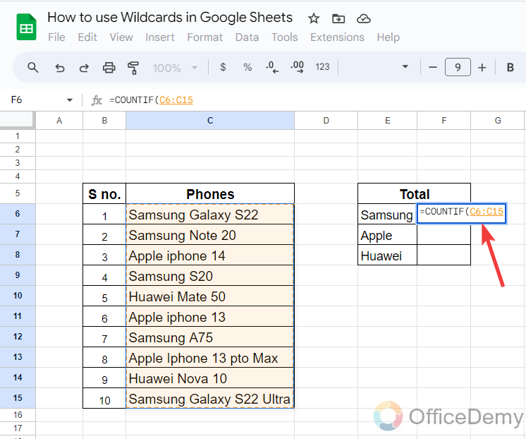
After starting the formula, first thing, we will provide the data range in which we are counting the data.

Step 4

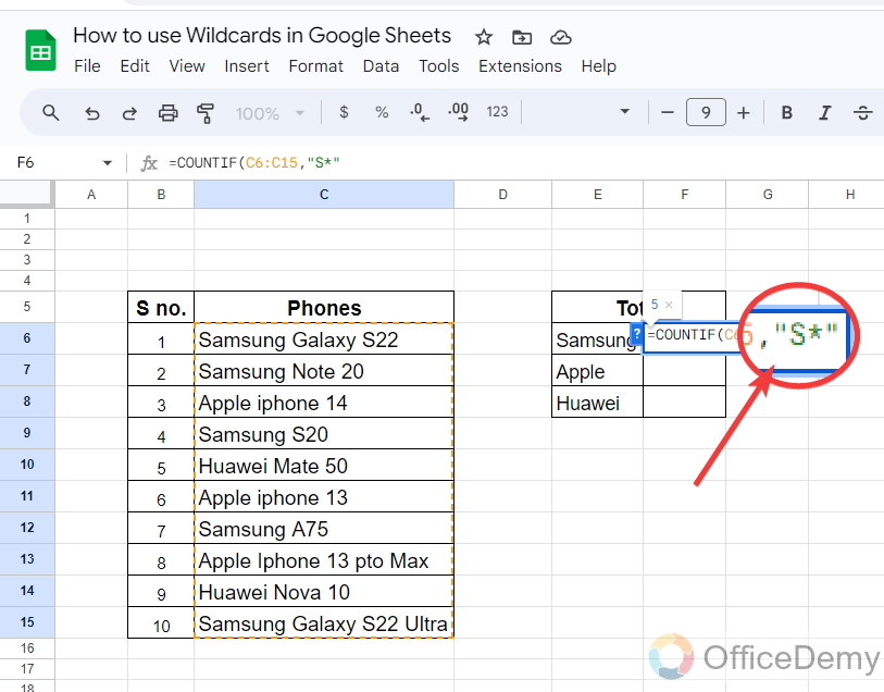
After giving the data range in the syntax, now it’s time to give the criteria, here we will use a wildcard as we know all Samsung mobiles start with the text “S“, so we can write “S*“.

Step 5

Now, just close the bracket and press the Enter key to get the result, in this way, Google Sheets will automatically count those cells that are starting from the “S” alphabet as given.

Step 6

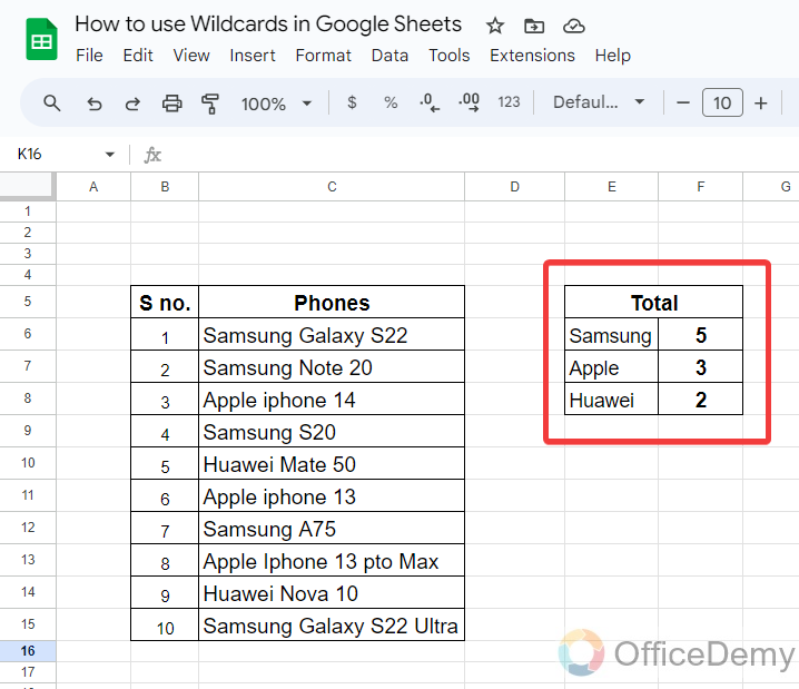
In the same, you can also find the quantity of all mobile phones of other brands as I have calculated in the following example.

Example # 2

In the same way, you can also use this wildcard in filtering data in Google Sheets. Let me show you with the help of the following steps.

Step 1

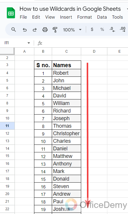
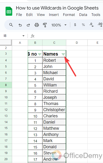
Let’s suppose, we have a table containing a huge list of names as you can see in the following sample data. Let me show you how can we use wildcards in filtering data.

Step 2

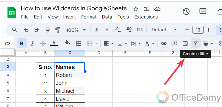
First, we will apply the filter on the column, to apply the filter select the cell where you want to apply the filter then click on the “Filter” icon as directed in the following picture.

Step 3

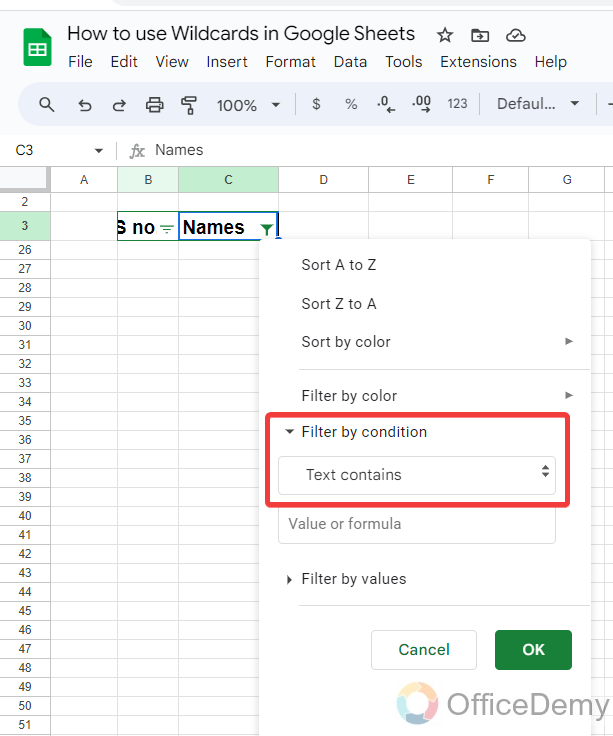
Once you have applied the filter, click on the filter option a drop-down menu will open where you will have to select the “Filter by condition” option as highlighted below.

Step 4

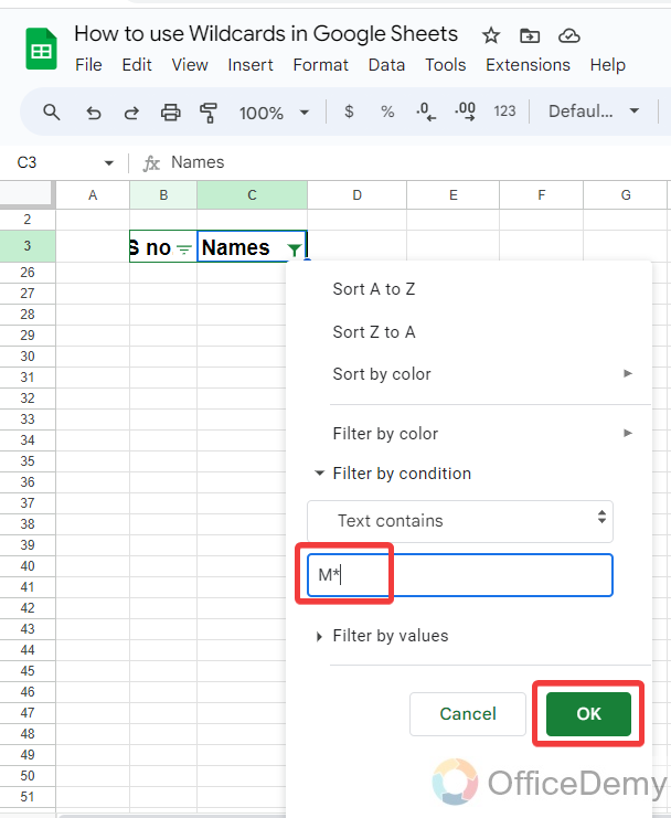
In the text dialogue box, write the condition “M*“, where the asterisk sign will work as a wildcard and enable you to find all those names containing the letter M. Let’s click on the “Ok” button to see the result.

Step 5

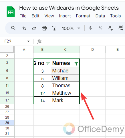
The result is in front of you, as you can see below all the names containing the letter M have been displayed in front of you. In the same way, you can filter your data with the help of a wildcard according to your needs.

How to Use Wildcards in Google Sheets – Question Mark (?)

A Question mark can only represent a single or one character or symbol in Google Sheets as a wildcard. Let’s suppose, if you know a word containing four letters in it and you remember just the first and last character then you can use two Question marks as a wildcard between the first and last letter to find the word. Go through the following examples to understand better.

Example # 1

Step 1

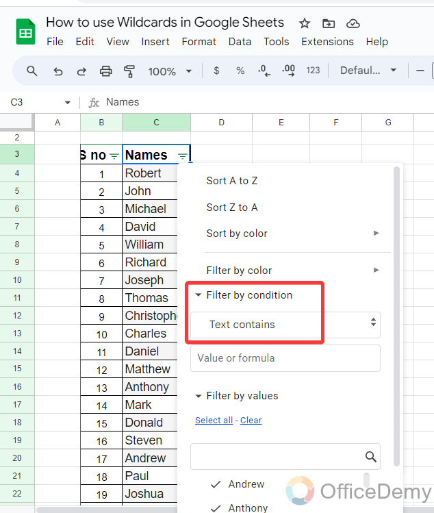
In this example, we will use the same sample data, let’s click on the filter option to apply filter criteria with the help of using a wildcard.

Step 2

When you click on the “Filter” icon, a drop-down menu will open where you will have to select the “Filter by condition” option and select the rule of “Text contains”

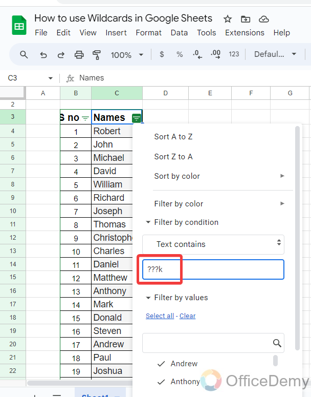
Step 3

Now, we will give the criteria to filter data where we will use wildcards, in the following screenshot, you see, I have written “???k” in the text box. It will find the word that contains three unknown words before the letter K.

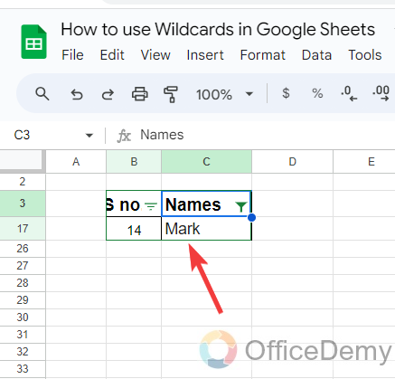
Step 4

As you can see the result in the following picture, it has searched the word that contains three letters before the letter K in the list.

Example # 2

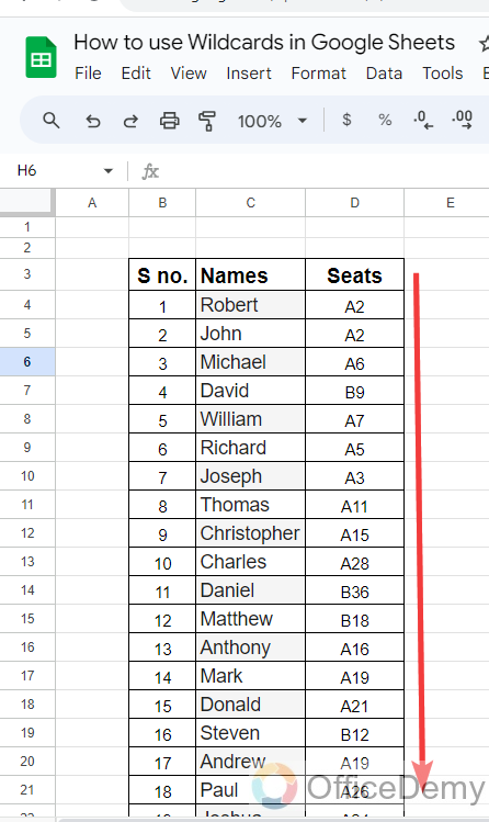
Step 1

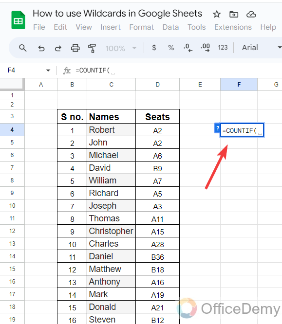
In the following example, we have a list of names with their seat codes for an exam. Let’s suppose, we need to count all those students whose seat numbers start with the letter B, but if we don’t know the exact seat number then you can count with the help of a wildcard. Let me show it practically in the following steps.

Step 2

To count seat numbers, we will use the COUNTIF formula as written below.

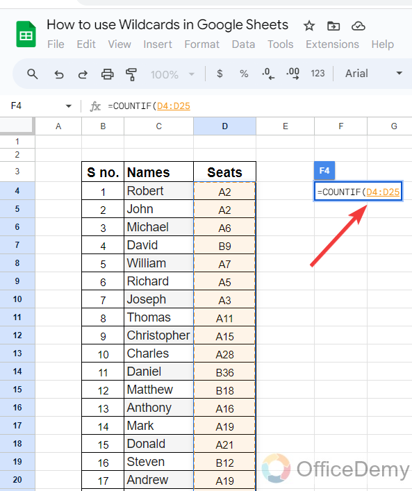
Step 3

After starting the formula here, first, we will give the data range of the seat numbers as we are counting seat numbers starting with the letter B.

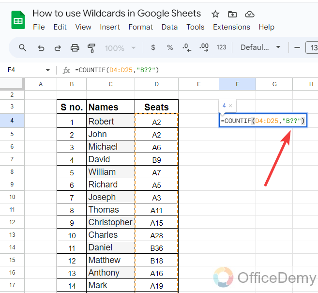
Step 4

After giving the data range, we will have to specify the criteria that we are looking for, we will write “B??“, as we only know that the seat numbers start with the letter B, and having two more characters for that I will use wildcard so, Google Sheets will automatically search for the given criteria.

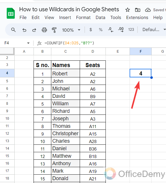
Step 5

As press the “Enter” key, we will get the result as can be seen in the following picture. In the same way, you find any query with even half information.

How to Use Wildcards in Google Sheets – Tilde (~)

Tilde in Google Sheets is very rarely used when your query is regarding an asterisk and Question mark that are already wildcards in Google Sheets so it is used to indicate that the proceeding character shouldn’t be considered as a wildcard. Overview the following examples so you may get the ideology of Tilde wildcard in Google Sheets.

Example # 1

Step 1

In the following example, we have a small sample data where we have to calculate the cells that contain “?” in it. Let’s see, what to do to count these cells.

Step 2

To count cells here we will use the “COUNTIF” formula as I have written in the following picture.

Step 3

After starting the formula of COUNTIF, first, we will have to provide the data range in which we are calculating the cells.

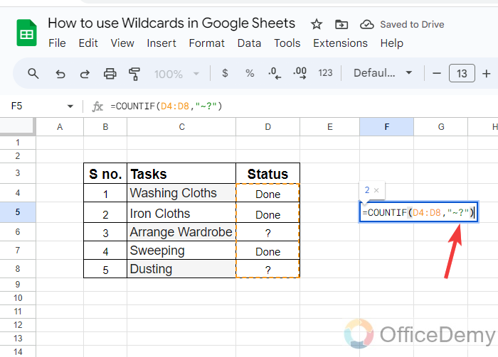
Step 4

After giving the data range, the next argument of the syntax will be the criteria that we are looking for, so here we will write the following pattern “~?” because a “?” is already a wildcard so in such a situation we use another wildcard “~” to get the result.

Example # 2

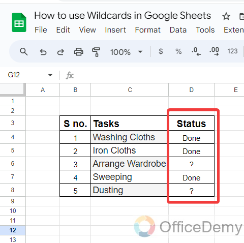
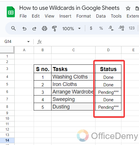
Step 1

Similarly, if you see in the following example, we have some tasks that are pending and written in the following pattern. To count pending tasks what will have to do? Let’s see.

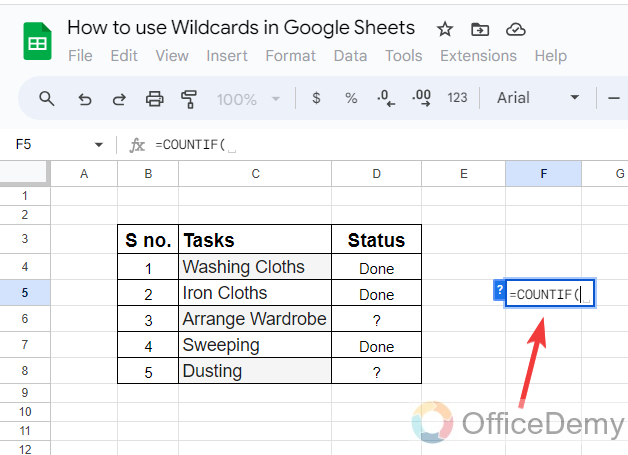
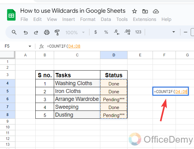
Step 2

Simply, first, we will run the COUNTIF function and then will give the data range as written below.

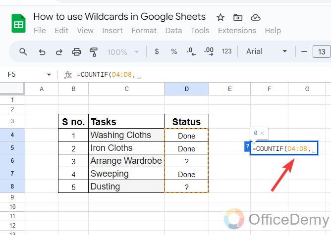
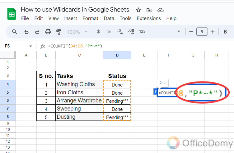
Step 3

After giving the data range, to specify the criteria, we will write in the following pattern “P*~*“. That will indicate that the text starts with the letter P has several letters and ends with the asterisk.

Step 4

If you only give the following criteria that “P*“, that will only detect the text that starts with the letter P and has several letters but will detect that it ends at the asterisk.

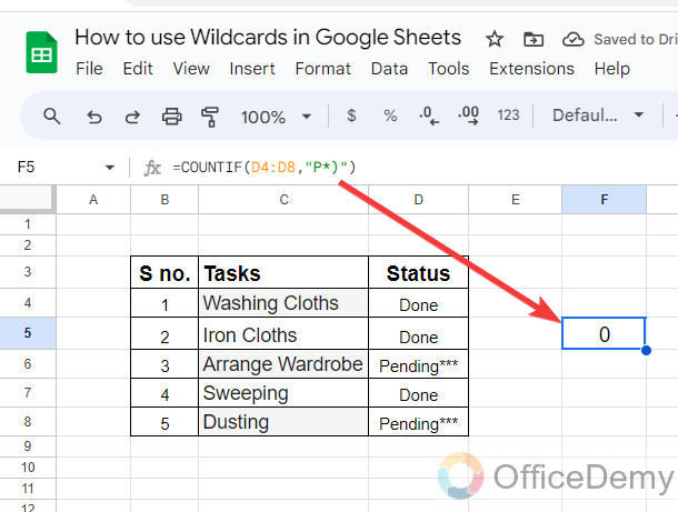
In such a situation we use tilde.

Frequently Asked Questions

Conclusion

As we have seen in the above article on how to use wildcards in Google Sheets, wildcards are the best way to search unknown text, or in various scenarios, we can use these wildcards when we have incomplete information. Hope, this practice will be helpful to you