How to Apply Conditional Formatting IF Box is Checked in Google Sheets

In this article we will learn about how to apply Conditional Formatting if box is checked in Google Sheets with real life example.

What is Conditional Formatting if box is checked Google Sheets

Checkboxes provide an easy way to keep the entries with True or False, Yes or No types of format. Using checkboxes, one just need to click on the box to check (True) and leaving it unchecked means false.

Google Sheets also provide this special feature making Google Sheets more interactive. We might further need to apply Conditional Formatting if box is checked Google Sheets. In this article, we will discuss how to apply Conditional Formatting if box is checked Google Sheets.

If you are interested to learn about How to Use Google Sheets Conditional Formatting Based on Another Column, please read the below article.

How to Use Google Sheets Conditional Formatting Based on Another Column

Why we use Conditional Formatting if box is checked Google Sheets

There are all sorts of problems when you start dealing with a large sum of data. Sometimes the problem can be to arrange a large sum of data based on the value of checkboxes.

For example, a tour management society may only consider the visitors who are vaccinated, or an institute might ignore the students who have foreign nationality for certain scholarships, etc. In order to solve these kinds of problems, we use checkboxes in Google Sheets and based on the value provided inside the Box, we can easily apply Conditional Formatting if box is checked Google Sheets using the method below.

Download/Copy Practice Workbook

How to apply Conditional Formatting if box is checked Google Sheets

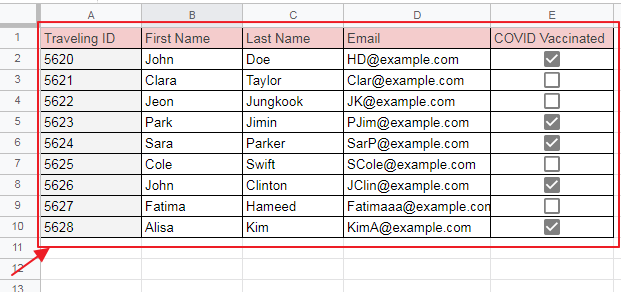
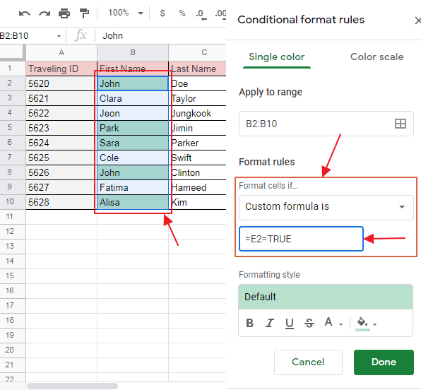
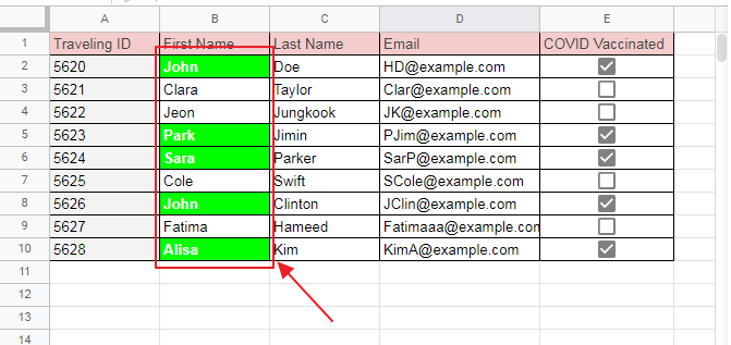
Suppose we have the following sheet consisting of the data of some Travelling Agency. They have some candidates, but they would only consider the candidates who are vaccinated and ignore/postpone travelling for the rest of candidates of travel. They want to filter out the traveling ID of candidates with highlighting First Name in green so that they can contact those candidates for further details.

[Every formatting will depend on its problem statement and requirements]

Step 1:

First of all, select those cells which have to be formatted.

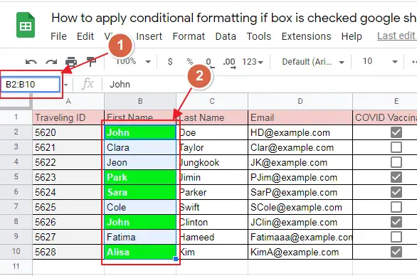
In this case, we will select the cells of column Traveling ID which are to be formatted according to the status of checkboxes.

Selected cells will appear in blue as:

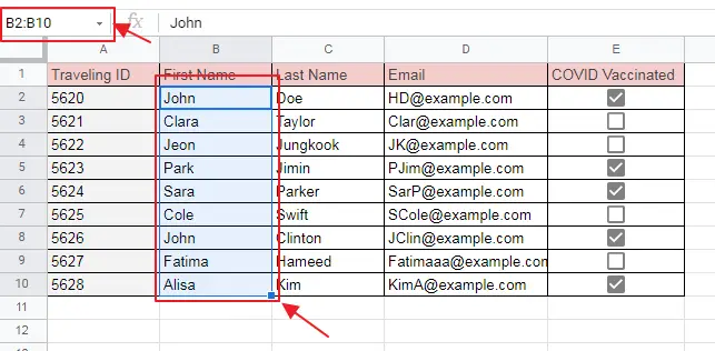
You can also see the cell numbers selected (displayed as a range) in top left corner.

Step 2:

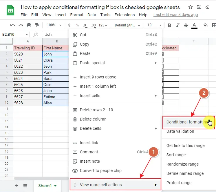
Now right click on selected area, a sub-menu will appear. Choose “View more cell actions”, and then “Conditional Formatting” as below:

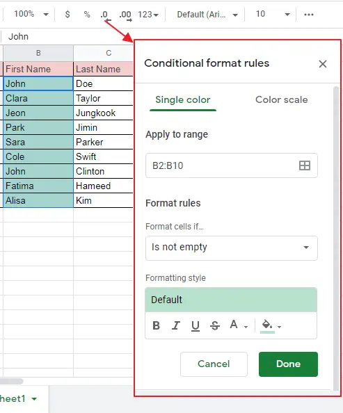
Conditional Format Rules Box will appear so you can now enter the set of rules for the required formatting.

Step 3:

Now set the formatting rules.

First of all, select from Format Rules, “Custom Formula is”, as shown below:

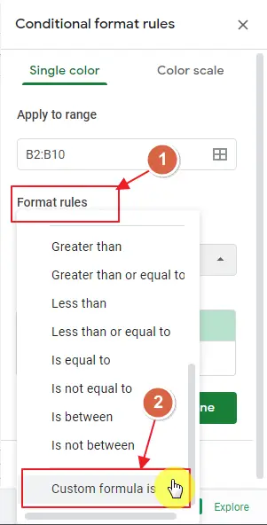
You will see that input box for inputting formula will appear right below as:

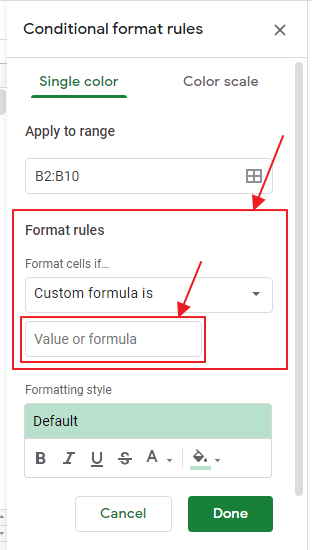
Write down the formula that is required to activate the Conditional Formatting later based on specific condition.

In this case, we need a special (conditional) formatting for the travelers first names to highlight using green highlight to visually imply that the specific traveler is eligible for travel.

So, formula here will be written as “=E2=TRUE”. It implies that as long as E2 is true (checkbox is checked), it satisfies the condition of Conditional Formatting and Conditional Formatting is applied.

Write down the formula as below and you will see the changes applying side by side as:

Step 4:

Now that you are done with writing the condition for Conditional Formatting, the next step is to set Formatting Style for Conditional Formatting.

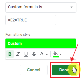
In this case, our motivation is to highlight the cells satisfying the condition, in Green. In this case, we will apply the Formatting style as:

You can always choose the formatting style as per the requirements.

Step 5:

Click “Done” to submit that conditional formatting has been applied.

You will see the conditional formatting is applied to the cells as:

Tutorial: Conditional Formatting if box is checked Google Sheets

Notes

Most of the times, we are dealing with a large set of data and cells, so it is not always possible to manually select the range of cells that are required to be formatted. Plus, this manual method is risky as we might mistakenly select an unrequired cell. So, the solution here is to select the range of cells by providing the cell numbers.

You can also select a range of cells by typing in the first cell of the range and then “:” implying that select the cells between (inclusive) first and the last cell in the upper left corner at:

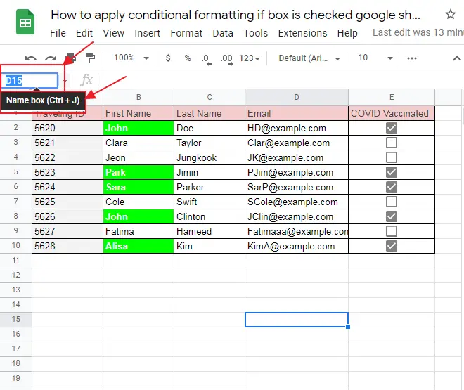
Now type in the required range as soon as you press “Enter”, you will see the given range is selected and appear in blue as:

Now, you can perform your desired actions on it as per requirements.

Conclusion

Checkboxes makes it easy to manipulate cells according to true of false (Yes or No) type of information. So, they are applied on the places when we are dealing with discrete Yes or No type of information, for example, Vaccinated? Eligible? Applied Earlier? types of fields. Method to applying conditional formatting if box is checked is explained in very easy manner. The steps are briefly elaborated above. If you have any issue with applying Conditional Formatting if Box is Checked Google Sheets or have any question, feel free to ask in comments section below.

Thanks for reading!