How to Use Google Sheets Conditional Formatting Multiple Columns

In this article we will learn about what is google sheets conditional formatting multiple columns and how to use it in real life with example and practice workbook.

What is Google Sheets Conditional Formatting Multiple Columns

Google Sheets Conditional Formatting Multiple Columns allows to conditionally format multiple columns of a sheet at a time. Conditional Formatting allows users to format the cells based on certain conditions to automatically carry out the procedure and save lots of precious time of its user. We might need to apply Conditional Formatting to more than one (multiple) columns of a sheet altogether for some specific purposes. In this article, we will discuss how to apply Google Sheets Conditional Formatting on Multiple Columns as a step by step procedure.

Why we use Google Sheets Conditional Formatting Multiple Columns

Sometimes the requirement of the problem may be to figure out or highlight certain cells within multiple columns. For example, a teacher may need to highlight cells having no marks as absent students on exam day. Performing this manually has its own risks. So using Google Sheets Conditional Formatting on Multiple Columns is the best approach here.

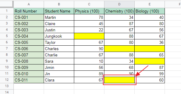
Let us say we have the following worksheet and we need to highlight the empty cells as absent students on the day of exam.

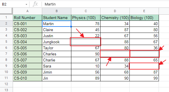
Also we need to make sure that extra cells in the columns, here Row 12 and ahead, do not highlight as they do not have student allocation in them. So we will use specific conditional formatting alongside using the formulae that makes the Conditional Formatting ignore the cells having no student allocated in it.

Download/Copy Practice Workbook

How to Do Google Sheets Conditional Formatting Multiple Columns?

Step 1:

Open the worksheet where you want to apply Conditional Formatting.

Step 2:

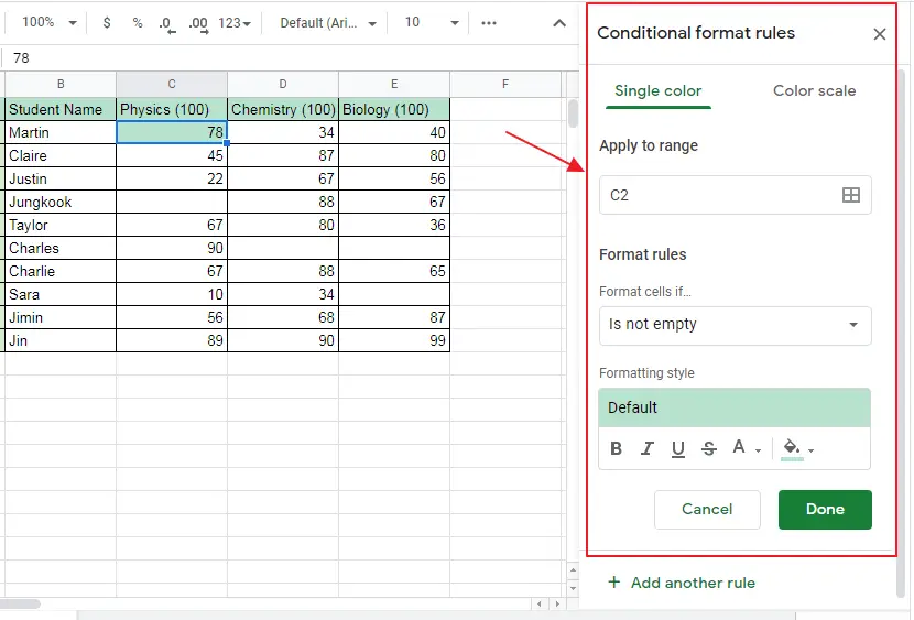
Click on Format from toolbar and select Conditional Formatting as shown below:

It does not matter which cell was selected at this time while applying conditional formatting because we are going to select and change the range of cell where Conditional Formatting will be applied manually.

Conditional Formatting Rules Box will appear as:

Step 3:

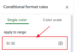
Now select the range of columns where Conditional Formatting needs to be applied.

Here we see that column C to E are to be formatted, so we describe the range as:

Step 4:

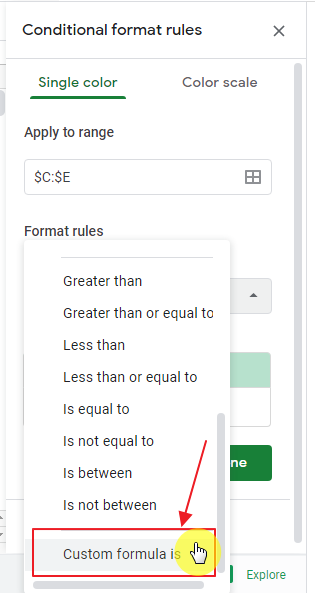
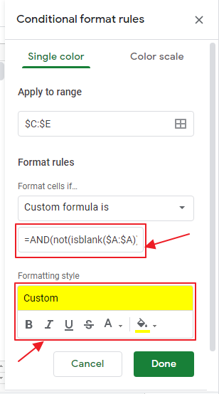
Describe Formatting Rules.

Here Formatting rules are a custom formula so we have to select “Custom Formula Is” from Format Rules as:

Now write down the formula in the box to describe the condition. Here condition is that Roll Number Column must not be empty and cell between C to E must be empty for highlighting.

So the formula can be written as

And apply the formatting style required for highlighting as:

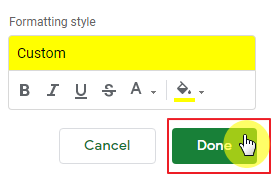
Step 5:

Click “Done” at the bottom of Conditional Formatting rules box.

Conditional Formatting throughout the columns will appear as:

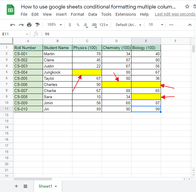
We can see that it clearly highlights the blank cells in the columns.

Now let’s say another record of a student is added as:

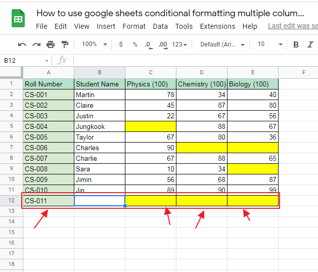
Just as Enter is pressed for submitting the roll number of a new entry of student, columns C:E are highlighted showing that desirable scenario has been achieved.

Now when we enter the entries of these columns, Sheets will automatically conditionally apply the formatting wherever required as:

Notes

Isblank() function returns true if the cell(s) value given in its parameters is blank. And returns false if cell(s) has some value in it.

In the above formula, isblank() function checks the value of column A. If A column has some value, it returns false. Not() function is applied on it which reverses true to false and false to true. AND function is applied over it describing that if and only if Column A’s cell contains some value and corresponding cells of range C:E are empty (contain no value) only then conditional formatting is applied.

It helps to avoid and ignore the cells which do not have student entry in them. Also as we checked above, if new students are added to the worksheet, Google Sheets automatically provide the formatting according to applied rules and conditions.

Frequently Asked Questions

What Are Some Ways to Compare Multiple Columns in Google Sheets?

When using Google Sheets, comparing columns in google sheets can be done in several ways. One method is to use the IF function combined with the VLOOKUP function to check for matching values between columns. Another option is to use the COUNTIF function to count the number of matching values in different columns. Additionally, the FILTER function can be used to display only the matching values between multiple columns. These techniques provide a quick and efficient way to compare multiple columns in Google Sheets.

Conclusion

Google Sheets provide the easy procedure for handling requirements of the worksheets so users need not to spend too much time to perform tasks that are better performed when automated and saves precious time of users. In this article, we studied easy, fast and step by step procedure for How to use google sheets conditional formatting on multiple columns. If there is any query or question about application of this method. Feel free to leave a comment below. We are more than happy to respond to your queries and reply to your messages.

Thanks for reading!