Conditional Formatting based on Another Cell in Google Sheets

In this article we will learn about How to use Conditional Formatting based on Another Cell in Google Sheets.

What is Conditional Formatting based on Another Cell in Google Sheets

Sometimes a user may need to perform certain formatting to a cell based on value on another cell in the sheet. This can be achieved by using Conditional Formatting based on Another Cell in Google Sheets. Google Sheets have made it easy to achieve it providing the conditional formatting rules. All we need to do is to write down the rule or condition that is required to activate the formatting. In this article, we will discuss easy and step-by-step method to achieve Conditional Formatting based on Another Cell in Google Sheets.

Why we use Conditional Formatting based on Another Cell in Google Sheets

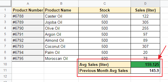
We might need to use Conditional Formatting based on Another Cell in Google Sheets for some specific problems such as we might need to highlight the product names whose sales are below average of all product sales. It is pretty difficult to work based on simple observation and analysis so it is always better to analyze while having highlighters pointed towards to cell(s) of focus. In this example, we have certain oils in stock and their per liter as well as average sale in liter for this month and also Average sales for the previous month as:

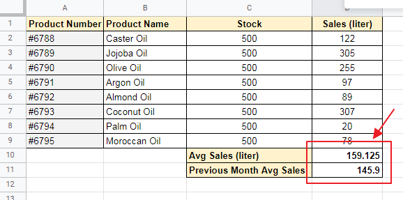
We have the average calculated through the use of formula and also previous month’s Average Sales (liter) is also available. Our task is to apply Conditional Formatting such that:

Download/Copy Practice Workbook

How to Do Conditional Formatting based on Another Cell in Google Sheets

Step 1:

Select the cell which needs to be formatted by clicking over it.

Here, select the cell showing current month’s Average Sales (Liter) as:

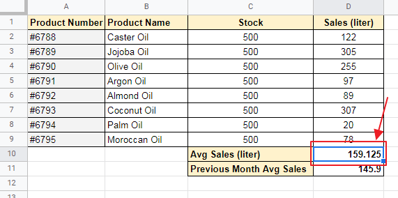
It will appear with a blue outline showing selection.

Step 2:

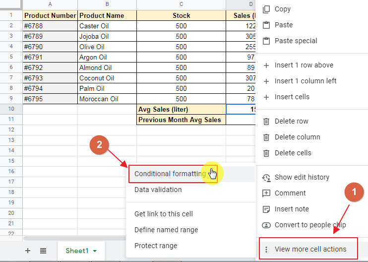
Apply Conditional Formatting either by

Right Click -> View More Cell Actions -> Conditional Formatting

Displayed as:

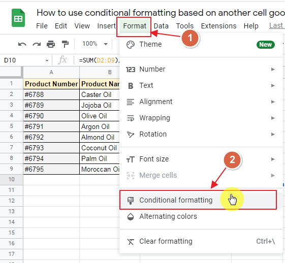
OR

You can also select Conditional Formatting from “Format” toolbar as:

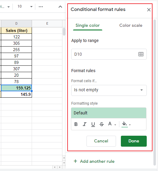
Conditional Formatting Rules Box will appear showing default conditional formatting as:

Step 3:

Apply Conditional Formatting Rules according to the requirements of your problem.

Here, we need to apply 2 rules as:

1. Average Sales of the current month is highlighted Blue if it is greater than Previous Month’s Average Sales.
2. Average Sales of the current month is highlighted Red if it is less than Previous Month’s Average Sales.

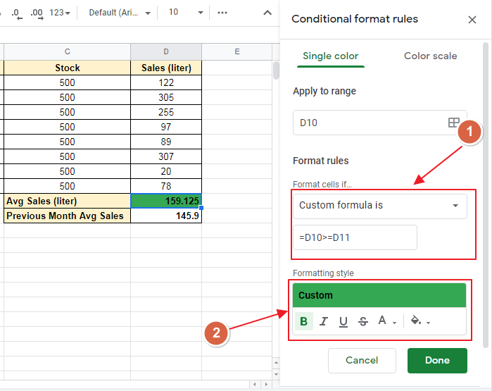
Rule 1 describes D10 must be greater than (or equals) D11 so we can write it as “=D10>=D11” and apply formatting as Green Highlight.

Select from Format Rules, Format cells if -> “Custom Formula Is” -> Write the formula “=D10>=D11” -> Apply Formatting Required (Highlight in green) as:

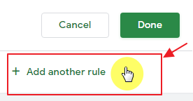
Also apply the second formatting rule for highlighting in red by choosing “Add another rule” as:

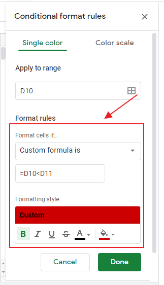
Now enter the rule details for next rule as:

Step 4:

Click “Done” using the button Done as:

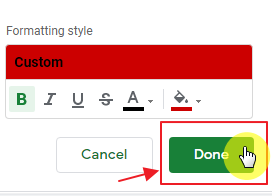
You can see the required Conditional Formatting is applied to the cell.

Notes

You can use Conditional Formatting based on Another Cell Google Sheets method for many other problems using other cell’s values or comparison between them to Conditionally Format another cell.

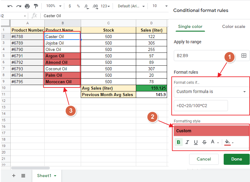
Make sure to use accurate value of cell number by checking in the cell name box for correct results. Also “=” sign describes the start of formula, if omitted the Conditional Formatting would not work properly. So using “=” sign is a must for using any formula. Here the formula is used to compare the values between current month’s average sale and previous month’s average sales. One similar problem can be to highlight the product names of the products whose sales are less than 20% of stock available. For product number #6788, formula will become “=D2<20/100*C2”. After applying this to whole column we have the result as:

To learn more about how to copy conditional formatting from one cell to others as used above, please refer to the article How to Copy Conditional Formatting in Google Sheets (2 Methods).

When you copy formatting from one cell to others (like above), relative addresses used in the formula are automatically calculated. It means that as the reference provided in the formula for B2 is B4 and B3, Google Sheets will automatically refer to the values of C4 and C3 for C2 cell conditional formatting and so on. User need not to do it manually and save a lot of time.

Frequently Asked Questions

How Can I Use the Lowest and Highest Value in Another Cell for Conditional Formatting in Google Sheets?

To use the lowest and highest conditional formatting values in another cell in Google Sheets, follow these steps. First, select the cell range where you want the conditional formatting to be applied. Then, from the Format menu, choose Conditional formatting. In the sidebar that appears, select Single color under the formatting style. Next, choose Custom formula is from the dropdown menu and enter the formula =A1=min(A:A) for the lowest value or =A1=max(A:A) for the highest value. Finally, set the desired formatting and click Done.

Can I Use Conditional Formatting in Google Sheets Based on Another Column?

Conclusion

The method for Conditional Formatting based on Another Cell Google Sheets is made easy and step-by-step elaborated procedure is given above. If there is any question, we would love to respond to it. Feel free to ask in the comment section below.

Thanks for reading!