
To Apply Conditional Formatting to Find Duplicates in Google Sheets
- Select the cells.
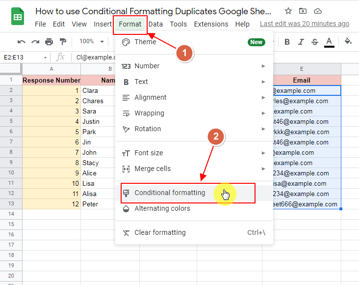
- Go to “Format” in the toolbar and choose “Conditional Formatting“.
- Set the condition as a custom formula.
- Use “=COUNTIF($E$2:$E$13,E2)>1” to find duplicates in the Email Column (modify the range as needed).
- Choose the desired formatting.
- Click “Done” to apply.
In this article we will learn about How to use Conditional Formatting Duplicates in Google Sheets and its use cases.
What is Conditional Formatting Duplicates Google Sheets?
Conditional Formatting provides an easy way to automatically format the Google Sheets by applying a formula or condition to be satisfied in order to activate Conditional Formatting. Conditional Formatting has a special feature using which we can find duplicates (duplicates of value of cells) in Google Sheets.
Sometimes we may face a problem where we have to find out the values which are duplicates of each other in a Google Sheet. Finding the duplicates manually may take hours. Here, in order to solve such problem with a few clicks, Google Sheets allow us to use Conditional Formatting Duplicates Google Sheets method. In this article, we will provide an easy method to use Conditional Formatting Duplicates Google Sheets.
Why we use Conditional Formatting Duplicates Google Sheets?
Sometimes, while working with Google Sheets, we may be dealing with a large amount of data set and required to find its validity in the terms of uniqueness. We are mostly dealing with large amounts of data and that data is input very carefully later it is not possible to check for uniqueness in a data set of thousands.
So, in these types of cases, we might want to highlight the cells which contain same duplicate values to throw them out of our data set to make our data set more valid and unique in terms of values. So that our results are only based on actual real values and not duplicates.
These may include finding duplicates in Full Names, ID Number, Driving License Number, Phone, Address, Citizenship Number, or email, etc. Google Sheets allows us to use Conditional Formatting Duplicates Google Sheets to find duplicate values in sheets. Using the method for Go Conditional Formatting Duplicates Google Sheets, we can find out those cells which contain duplicate values and exterminate them and work only on actual values.
Download/Copy Practice Workbook
How to use Conditional Formatting Duplicates Google Sheets?
Let us take an example of a Google Sheet where Response List upon a Skin Product is provided. Here, the example contains only a few cells for demonstration. Actually, the data of responses may exceed hundreds of responses and then, it will become particularly difficult to find out the cells containing duplicate values and exclude those responses from response list as they are fake responses. Here we demonstrate the method on the sheet as below:
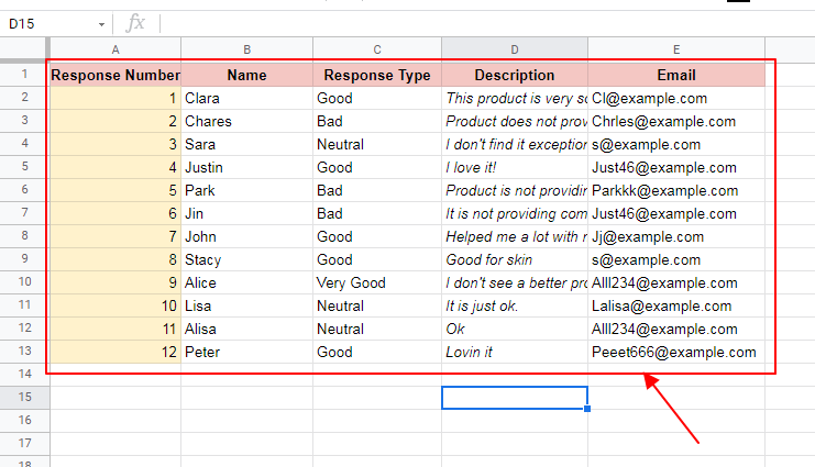
Now, we have to highlight the cells containing duplicate values in email column to exclude them.
Let us apply the Conditional Formatting Duplicates Google Sheets as following:
Step 1:
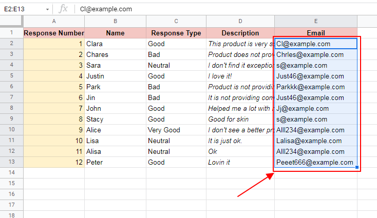
Select the cells where you want to apply the Conditional Formatting.
In this case, we need to apply the Conditional Formatting to the Email Column.
We can select manually by dragging the mouse over the required cells as:
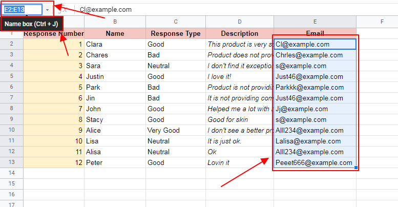
OR
We can type in the range of cells to conditionally format in “Name Box” as below:
As we select the cells, we see that the selected cells are highlighted in light blue showing selection.
Step 2:
Next step is to apply Conditional Formatting.
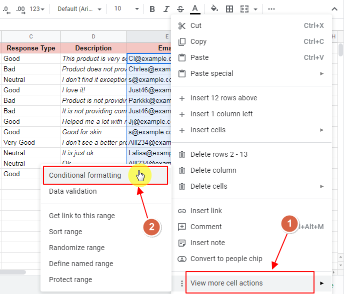
As the cells are selected, we can apply conditional formatting using any of the 2 methods below:
- Method 1:
- Right Click anywhere on the selected cells. A sub-menu will appear. Choose “View more cell actions” and then Conditional Formatting as shown below:
- Right Click -> View More Cell Actions -> Conditional Formatting
- Method 2:
- From the Format toolbar, choose Conditional Formatting as shown below:
- Format -> Conditional Formatting
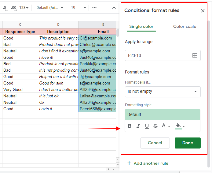
As we click on Conditional Formatting, Conditional Formatting Rules Box will appear as:
Step 3:
Set the condition that is required to activate the conditional formatting.
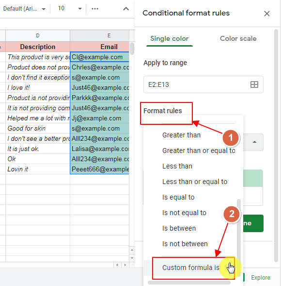
Here, we need to highlight the cells which are duplicates of each other. So, we apply the condition as a custom formula.
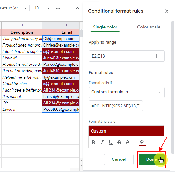
Apply custom formula by selecting the Custom Formula Is under the Format Rules section as:
Now type the formula in the Formula or Value Box in Format Rules section. In this case, the condition is to find out which cells are duplicates, so our formula here is =COUNTIF($E$2:$E$13,E2)>1. We apply it as:
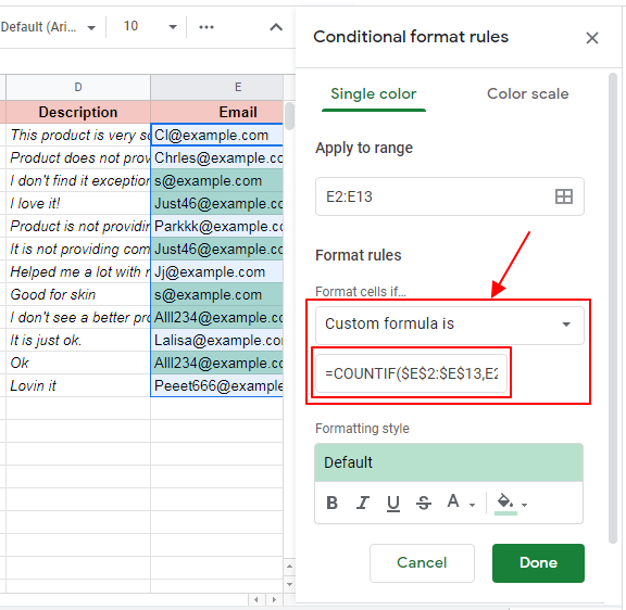
As soon as we apply the custom formula, we begin to see changes in our sheet.
Step 4:
Condition for Conditional Formatting is set, now is the time to set the “Format” for Conditional Formatting. We can set our required format in Formatting Style section in Conditional Format Rule Box as:

Step 5:
Click “Done” to submit the conditional formatting has been applied.
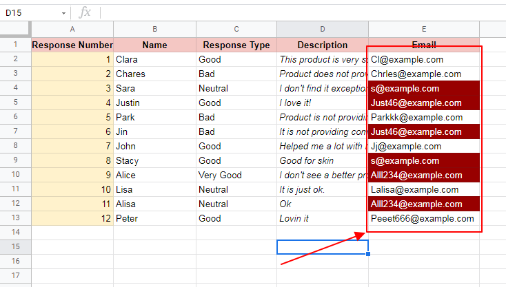
We can see the conditional formatting has been applied as:
We could also cancel the conditional formatting if we do not require this formatting by clicking cancel button.
We know from the above results that out of 12 responsive, 6 responses are fake and should be removed from the product reviews list.
Notes
We used the formula “=COUNTIF($E$2:$E$13,E2)>1” in this example. It can be changed as per requirements of the problem scenario. Remember that this formula contains absolute cell numbers and hence cannot be carelessly copy-pasted. Or copying conditional formatting with this formula would not be useful. So the user has to specify the range for the cells where duplicates are required to be found out very carefully specifying the absolute cell numbers.
Frequently Asked Questions
What Are the Different Methods for Finding and Highlighting Duplicates in Google Sheets?
Finding and highlighting duplicates in Google Sheets can be done using various methods. The built-in conditional formatting feature combined with custom formulas allows users to easily pinpoint repetitive data. By applying the google sheets duplicate highlight function, users can efficiently identify and manage duplicate entries in their spreadsheets with just a few simple steps.
Can I Use Conditional Formatting to Find Duplicates in Google Sheets If the Cells Contain Formulas?
Yes, you can use conditional formatting for cell formulas in Google Sheets to find duplicates. This feature allows you to set up rules that will highlight any duplicate values within the specified range. By applying the conditional formatting rule with the keyword conditional formatting for cell formulas, you can quickly identify and manage duplicates in your spreadsheet.
Conclusion
Applying Conditional Formatting Duplicates Google Sheets allows us to find duplicate cells in large sheets which enables us to clear duplicates and find unique values in our sheets and save the data set from duplication and false values. In this article, easy step-by-step method for Conditional Formatting Duplicates Google Sheets is described. Any queries are most welcomed. Feel free to comment below for any questions.
Thanks for Reading!


