How to Group Rows in Google Sheets [Best Practice]

The best way to Group Rows in Google Sheets: Select the rows you want to group > Right-click > “Group rows row (2) to row (6)” > Collapse the group by clicking the minus sign > To ungroup, right-click and select “Ungroup row (2) to row (6)“

In this article, we will learn how to group rows in google sheets.

Group rows in google sheets is the latest addition in Google Spreadsheet. Before this we used to perform row grouping using manual methods and custom formulas, but google has brought another exiting pre-defined feature for us that is called group rows and columns. We will see today. We will see how to group rows in google sheets.

So basically, group rows are nothing but grouping multiple rows together and get a button to expand and collapse over it. It helps us a lot when we are working on a large data. It helps us collapsing all the detailed view and keep only important figures expanded to increase the clarity and readability. Further we will see its uses and how to use it in step-by-step procedure below.

Table of Contents

Importance of grouping rows in google sheets?

In google sheets we may have huge documents, like Order sheets, student’s records, patient records, production summaries etc. This kind of data is maintained daily and have some addition of data on regular basis. These files are way too detailed at the end of month. So, to make it more presentable and precise when presenting to our boss/client, we should take care of preciseness and clarity.

Here we can use group rows feature to keep all unnecessary details hidden and all the important values, and summaries on the front. We have a clickable “+” and “-” button to expand/collapse these groups in single click.

To hide details and only make visible the important figures.
To increase document clarity and readability.
To make our data more readable and user-friendly.

How to Group Rows in Google Sheets

Step 1

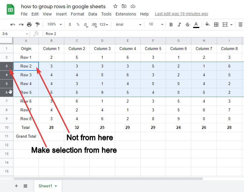
Select the rows from their parent header.

Step 2

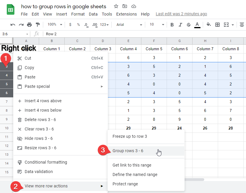
Right-click anywhere in the selected area go to view more row actions > group rows row (2) to row (6). 1 and 3 are the number of rows, they vary according to the row number.

Step 3

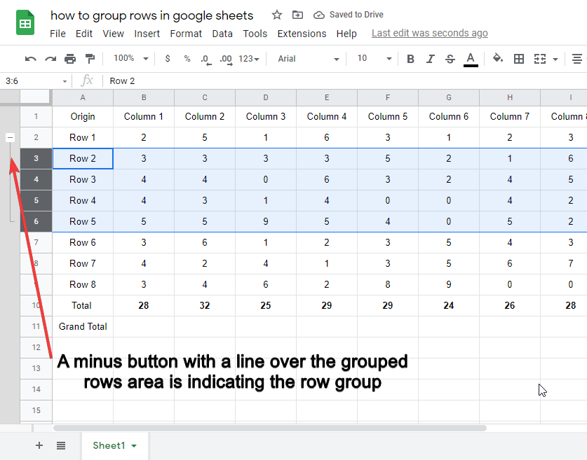
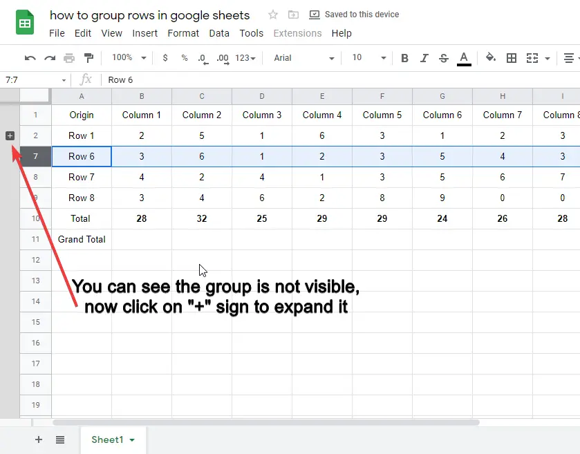
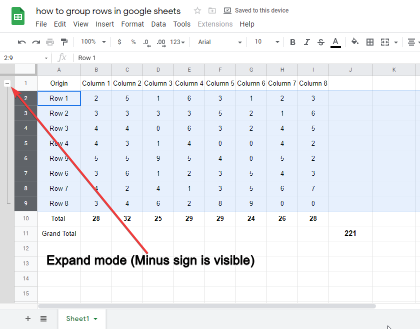
Rows have been groups; you can see a minus sign and a thin line at the left more corner. Click on the minus sign to collapse the group.

Step 4

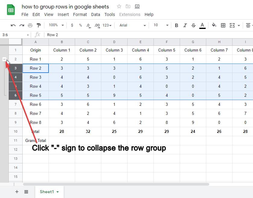
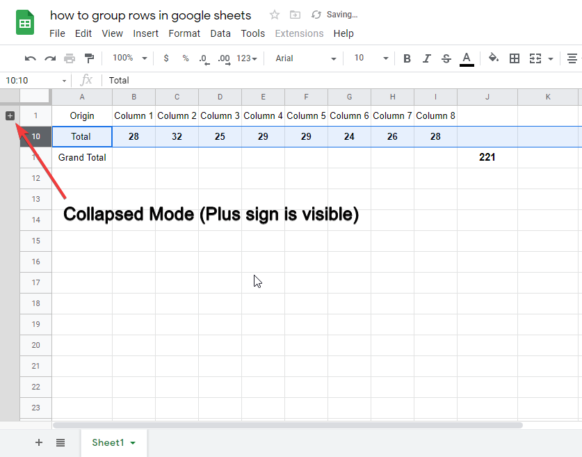
You can collapse the group by clicking on the minus – button. The minus sign will become a plus + sign that will indicate that the group is currently collapsed.

Step 5

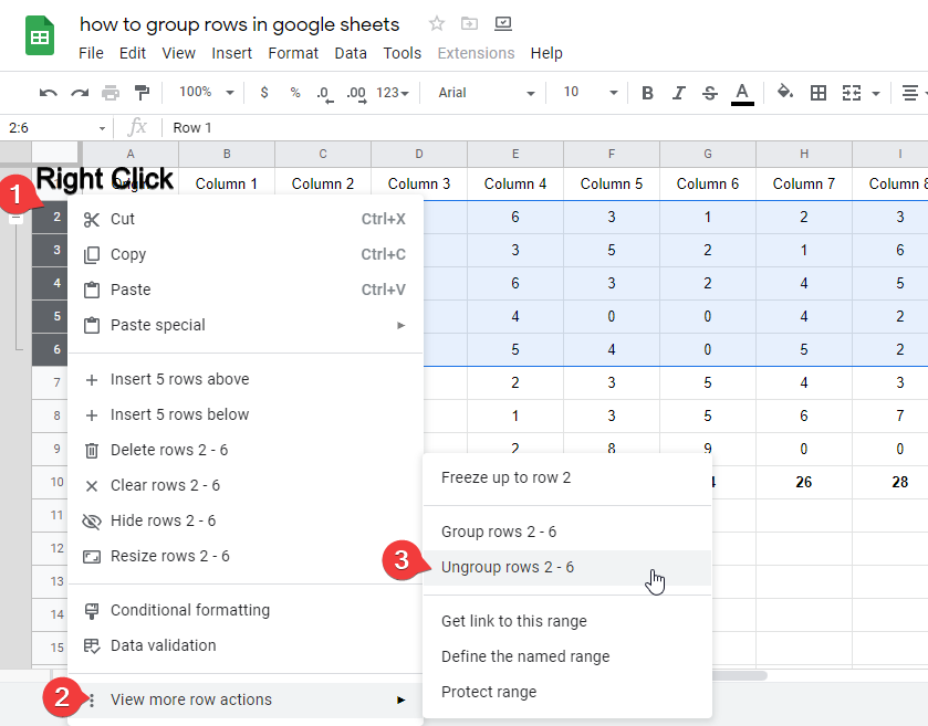
You can ungroup rows, by right selecting the grouped rows, right-click, view more row actions > ungroup row (2) to row (6).

Step 6 (Optional)

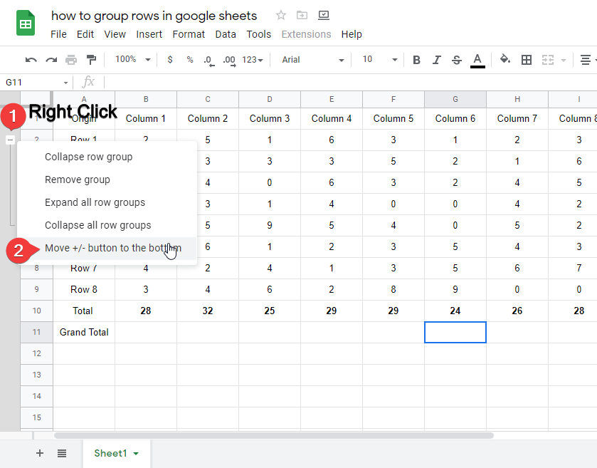
You can move your “+”,”-” sign for your ease by doing a right-click on the button and clicking on the “Move +/- button to bottom/top”.

Tips

You can use nested groups to add multiple buttons, and you can make all rows group excluding the total to make only the total visible in collapsed mode.

To recap, we learned how to group rows in google sheets, it is a simple feature but very useful and can be a big lifesaver when it comes to presenting your data to your boss/client. We learned how can we use it to make our data precise and highly readable. We also discussed the reasons where we need to use row groups in google sheets. We discussed 5 important steps and one optional step. Follow the steps properly and practice it you become an expert in group rows in google sheets.

Important Notes

Always remember that selection will be done from the left-most parent headers of the rows.
If you select the rows from anywhere else, the selection will be made but you will not be able to find the group row option.
Try to make organized groups, don’t make it messy, always make sub-groups and then a master group to keep a conceptual hierarchy.

Frequently Asked Questions

Is it Necessary to Resize Rows and Columns before Grouping in Google Sheets?

Before grouping data in Google Sheets, it is essential to resize rows and columns. This ensures that the grouped sections are organized and visually appealing. When rows and columns are properly adjusted, it becomes easier to analyze and interpret the data within each group. Therefore, resizing rows and columns is necessary for effective grouping in Google Sheets.

Conclusion

In this article, we learned how to group rows in google sheets. It’s not one of the most difficult features in google sheets but essentially, it’s very useful and maybe a little tricky in the beginning. Google sheets are becoming very powerful and adapting more programmatical scripts and formulas to allow users to perform their tasks very accurately. Group rows feature is recently added in google sheets, and you can easily master it by following our 5 steps guide. We have covered everything from beginning to advance. So, if you like this article then consider subscribing to our OfficeDemy blogs, also do share this article with your friends.